Problem 12.9

Fundamentals of Solar Cells and Photovoltaic Systems Engineering

Solutions Manual - Chapter 12

Problem 12.9

When the spectral response of the reference cell is different from the cell under test and/or the spectrum of the simulator lamp is different from the reference spectrum, the spectral mismatch factor \(M_f\) can be used to correct the measurement. In this problem, the QE of a GaInP cell (device under test) and a calibrated Si solar cell (reference cell) are provided. Calculate their respective SR and estimate the corresponding spectral mismatch factor, when the test cell is measured using a quartz tungsten halogen lamp, relative to the reference spectrum AM1.5 G.

We will use the package pandas to handle the data and matplotlib.pyplot to plot the results.

import pandas as pd
import numpy as np
import matplotlib.pyplot as plt

We start by importing the data for the solar spectra.

reference = pd.read_csv('data/Reference_spectrum_ASTM-G173-03.csv', index_col=0, header=0) 
reference

	AM0	AM1.5G	AM1.5D
Wvlgth nm	Etr W*m-2*nm-1	Global tilt W*m-2*nm-1	Direct+circumsolar W*m-2*nm-1
280	8.20E-02	4.73E-23	2.54E-26
280.5	9.90E-02	1.23E-21	1.09E-24
281	1.50E-01	5.69E-21	6.13E-24
281.5	2.12E-01	1.57E-19	2.75E-22
...	...	...	...
3980	8.84E-03	7.39E-03	7.40E-03
3985	8.80E-03	7.43E-03	7.45E-03
3990	8.78E-03	7.37E-03	7.39E-03
3995	8.70E-03	7.21E-03	7.23E-03
4000	8.68E-03	7.10E-03	7.12E-03

2003 rows × 3 columns

reference.drop(reference.index[0], inplace=True)   # remove row including information on units
reference=reference.astype(float)                  # convert values to float for easy operation
reference.index=reference.index.astype(float)      # convert indexes to float for easy operation

We import the data for the quartz tungsten halogen lamp.

quartz_w = pd.read_csv('data/W lamp spectral irradiance.csv', index_col=0, header=0) 
quartz_w

	W halogen lamp (W*m-2*nm-1)
wavelength (nm)
300	0.000001
301	0.000010
302	0.000100
303	0.000200
304	0.000300
...	...
1196	0.654304
1197	0.653941
1198	0.651544
1199	0.647531
1200	0.644677

901 rows × 1 columns

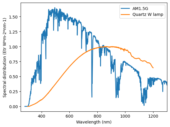
We can also plot the AM1.5G spectra and the quartz tungsten halogen lamp spectra.

plt.plot(reference['AM1.5G'], 
         linewidth=2, label='AM1.5G')
plt.plot(quartz_w['W halogen lamp (W*m-2*nm-1)'], 
         linewidth=2, label='Quartz W lamp')
plt.ylabel('Spectral distribution (Etr W*m-2*nm-1)')
plt.xlabel('Wavelength (nm)')
plt.xlim([250,1300])
plt.legend()

<matplotlib.legend.Legend at 0x7f9b34d1ba50>

We define the relevant constants and retrieve the QE of the GaInP solar cell (device under test), and the callibrated Silicon solar cell (reference cell).

h=6.63*10**(-34)   # [J·s] Planck constant
e=1.60*10**(-19)   # [C] electron charge
c =299792458       #[m/s] Light speed

QE_dut = pd.read_csv('data/QE_GaInP.csv', index_col=0, header=0) 
QE_cal= pd.read_csv('data/QE_calibrated_cell.csv', index_col=0, header=0) 

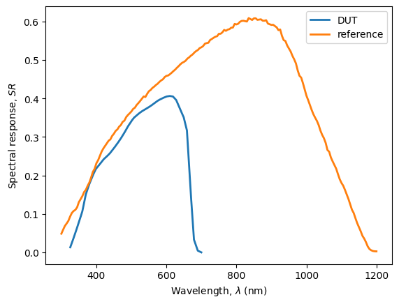
We calculate the Spectral Response (SR) of both cells and plot them.

SR_dut=pd.Series(index=QE_dut.index,
            data=[QE_dut.loc[i,'QE']*e*i*0.000000001/(h*c) for i in QE_dut.index])
SR_cal=pd.Series(index=QE_cal.index,
            data=[QE_cal.loc[i,'QE']*e*i*0.000000001/(h*c) for i in QE_cal.index])
plt.plot(SR_dut, 
         linewidth=2,
        label='DUT')
plt.plot(SR_cal, 
         linewidth=2,
        label='reference')
plt.legend()
plt.ylabel('Spectral response, $SR$')
plt.xlabel(r'Wavelength, $\lambda$ (nm)');

For every spectra and solar cell, we interpolate the spectrum at those datapoints included in the SR, and integrate to obtain the short-circuit current density using Eq. 3.5.

\(J_{L, spectrum, cell}=\int SR(\lambda) \cdot G(\lambda) \ d\lambda\)

spectra=quartz_w['W halogen lamp (W*m-2*nm-1)']
spectra_interpolated=np.interp(SR_dut.index, spectra.index, spectra.values)
J_sim_dut = np.trapz([x*y for x,y in zip(SR_dut, spectra_interpolated)], x=SR_dut.index)*1000/10000 # A-> mA ; m2 -> cm2
spectra_interpolated=np.interp(SR_cal.index, spectra.index, spectra.values)
J_sim_cal = np.trapz([x*y for x,y in zip(SR_cal, spectra_interpolated)], x=SR_cal.index)*1000/10000 # A-> mA ; m2 -> cm2

spectra=reference['AM1.5G']
spectra_interpolated=np.interp(SR_dut.index, spectra.index, spectra.values)
J_ref_dut =np.trapz([x*y for x,y in zip(SR_dut, spectra_interpolated)], x=SR_dut.index)*1000/10000 # A-> mA ; m2 -> cm2

spectra_interpolated=np.interp(SR_cal.index, spectra.index, spectra.values)
J_ref_cal =np.trapz([x*y for x,y in zip(SR_cal, spectra_interpolated)], x=SR_cal.index)*1000/10000 # A-> mA ; m2 -> cm2

We calculate the Spectral Mismatch Factor \(M_f\) using Eq. 12.2

\(M_f=\frac{J_{L, sim, dut}}{J_{L, ref, dut}}\frac{J_{L, ref, cal}}{J_{L, sim, cal}}\)

M_f=J_sim_dut/J_ref_dut*J_ref_cal/J_sim_cal
print('Spectral Mismatch Factor = ' + str(M_f.round(3)))

Spectral Mismatch Factor = 0.45