Problem 4.11

Fundamentals of Solar Cells and Photovoltaic Systems Engineering

Solutions Manual - Chapter 4

Problem 4.11

Using the same solar cell parameters of Problem S4.4 (with series resistance \(R_s\)=1mΩ and parallel resistance \(R_p\)=500 Ω),

(a) generate one I-V curve using a high number of datapoints (e.g., 500) and then extract the one-diode model parameters from it using the five-point method coded in the python notebook for this problem. Do the \(R_s\) and \(R_p\) extracted fit the actual values?

(b) Now decrease the number of datapoints in the I-V curve down to 50 and see how the extracted parameters vary. Why does that happen?

(c) Finally, increase the noise in the data and see how the extracted parameters vary. Explain why this happens and propose a way to mitigate this effect.

First, we import the Python modules used and define the Boltzman constant

import numpy as np
import matplotlib.pyplot as plt

kB = 8.617333e-5

We define the variables for the I-V curve data

# These are values in the usual range for a typical 16.6 x 16.6 cm2 Si solar cell
Isc = 10.0 # A
I0 = 2e-9 # A
Rs = 1e-3 # ohm
Rp = 500 # ohm
n = 1.2

temperature = 25  #ºC
cell_area = 16.6*16.6 # cm2

Function to generate I-V curves using as input the parameters of the one-diode model

# Input data: 
# · single-diode model parameters
# · temperature
# · noise in the current, defined as a normal distribution with std dev of I*Inoise
# · number of datapoints to use
def model_IV(IL, I0, n, Rs, Rp, temperature, Inoise, data_size):
    # Thermal voltage
    kBT = kB*(temperature + 273.15)
    
    #I-V curve stored in a 2-column array: first column for voltages, second column for currents
    IVcurve = np.zeros((data_size,2))
    
    # First we calculate the I-V curve voltage range: from -0.1 V to Voc + 0.01 V
    # We want to have the I-V curve crossing the current and voltage axis to see the Isc and Voc
    
    # To determine the voltage range, we calculate first the Voc without Rs/Rp.
    Voc0 = n*kBT*np.log(IL/I0)
    
    #Create the voltage list
    #Voltage range used: -0.1 to Voc+0.01
    #A "Rs*IL" term is added to compensate for the voltage drop in the Rs
    IVcurve[:,0]= np.linspace(-0.1+Rs*IL, Voc0+0.01, data_size)
    
    #I-V curve without Rs effect
    IVcurve[:,1]= IL - I0*(np.exp(IVcurve[:,0]/(n*kBT))-1) - IVcurve[:,0]/Rp
    
    #Shift voltages to include Rs effect
    IVcurve[:,0] = IVcurve[:,0] - Rs*IVcurve[:,1]
    
    # Add noise to the current.
    # The noise component follows a normal distribution with std dev of I*Inoise
    IVnoise = np.random.default_rng().normal(0, np.absolute(IVcurve[:,1])*Inoise)
    IVcurve[:,1]+=IVnoise
    
   
    return IVcurve

Function to extract the I-V curve parameters

The algorithm is from:

• Cotfas, D.T., Cotfas, P.A., Kaplanis, S., 2013. Methods to determine the dc parameters of solar cells: A critical review. Renew. Sustain. Energy Rev. 28, 588–596. https://doi.org/10.1016/j.rser.2013.08.017

Note that this function does not assume that the I-V curve is in the first quadrant.

Another two functions are used to calculate the Isc and Voc and detect the quadrant. Then, the function calculating Pmax moves the I-V curve to this quadrant, if it is not there yet.

# Input data:
# · experimental I-V curve
# · temperature
# · number of points around Isc to calculate the I-V slope
# · number of points around Voc to calculate the I-V slope

def get_IV_params(rawIV, temperature):
    # Thermal voltage
    kBT = 8.617333e-5*(temperature + 273.15)
    
    ## 1) Prepare the I-V curve to be in 1st quadrant and 
    ##    with increasing values of voltage
    # Move I-V curve to first quadrant if it is not there yet
    # Sort data and move to first quadrant
    IV_1stq = rawIV.copy()
    Isc = get_Isc(IV_1stq)
    if Isc<0:
        Isc*=-1
        IV_1stq[:,1]*=-1
    
    Voc = get_Voc(IV_1stq)
    if Voc<0:
        Voc*=-1
        IV_1stq[:,0]*=-1    

    # Sort I-V curve data to have increasing values of voltage
    IV_1stq=IV_1stq[IV_1stq[:,0].argsort()]     
    ##
    
    ## 2) Algorithm for the 5-point method
    ##
    
    # Calculate Rp as the inverse of the slope at V=0
    # The function "getSlope_atIsc" returns the slope and the linear function to be plotted later
    slopeIsc, slopeFitIsc = getSlope_atIsc(IV_1stq)
    Rp = -1/slopeIsc
   
     # Calculate the maximum power and V, I at maximum power point
    Pm, Vm, Im = get_Pmax(rawIV)
    
    # Calculate the slope at Voc as intermediate parameter
    # The function "getSlope_atVoc" returns the slope and the linear function to be plotted later
    slopeVoc, slopeFitVoc = getSlope_atVoc(IV_1stq)
    
    # Intermediate calculations in the 5-point algorithm
    Rs0 = -1/slopeVoc
    
    A = Vm + Rs0*Im-Voc
    B = np.log(Isc-Vm/Rp-Im)-np.log(Isc-Voc/Rp)
    C = Im/(Isc-Voc/Rp)
    n = A/(kBT*(B+C))    
    
    I0 = (Isc-Voc/Rp)*np.exp(-Voc/(n*kBT))
  
    Rs = Rs0 -n*(kBT/I0)*np.exp(-Voc/(n*kBT))
   
    IL = Isc*(1+Rs/Rp) + I0*(np.exp(Isc*Rs/(n*kBT))-1)


    return IL, I0, n, Rs, Rp, slopeFitIsc, slopeFitVoc

And ancillary functions to serve “get_IV_params”

# Obtains Isc by linear interpolation around V=0
def get_Isc(IVdata):
    """Returns the Isc of the input raw I-V curve"""

   # Sort data
    IV_sorted = IVdata.copy()
    IV_sorted=IVdata[IVdata[:,0].argsort()]   # Sort by voltages
    
    Isc = np.interp(0,IV_sorted[:,0],IV_sorted[:,1])
    
    return Isc

# Obtains Voc by linear interpolation around I=0
def get_Voc(IVdata):
    """Returns the Voc of the input raw I-V curve"""

   # Sort data
    IV_sorted = IVdata.copy()
    IV_sorted=IVdata[IVdata[:,1].argsort()]   # Sort by currents
    
    Voc = np.interp(0, IV_sorted[:,1],IV_sorted[:,0])
    
    return Voc

# Obtains the Pmax, and also the Vm and Im
def get_Pmax(IVdata):
  
   # Sort data and move to 1st quadrant
    IV_sorted = IVdata.copy()
 
    Isc = get_Isc(IV_sorted)
    if Isc<0:
        Isc*=-1
        IV_sorted[:,1]*=-1
    
    Voc = get_Voc(IV_sorted)
    if Voc<0:
        Voc*=-1
        IV_sorted[:,0]*=-1       
 
    IV_sorted=IV_sorted[IV_sorted[:,0].argsort()]   
   
 
    PV = IV_sorted.copy()
    PV[:,1] = IV_sorted[:,0]*IV_sorted[:,1]
    
    Pm = np.amax(PV[:,1])
    maxPosition = np.argmax(PV[:,1])
    Vm = PV[maxPosition,0]
    Im = IV_sorted[maxPosition,1]

    return Pm, Vm, Im

# Determines the slope of the I-V curve around Voc
# I-V curve is assumed to be in 1st quadrant
def getSlope_atVoc(data):
  
    # Find the first negative current point
    # Determine the range for the fit according to nPnts
    rI = np.where(data[:,1] <= 0)
    rangeI = np.asarray(rI)  
    rangeI = rangeI.flatten()   
    
    indexEnd = rangeI[0] + 2
    if indexEnd > len(data[:,0])-1:
        indexEnd = len(data[:,0])-1
    indexStart = rangeI[0] - 2
    if indexStart < 0:
        indexStart=0
    
    # Fit to a polynomial of degree 1
    polyCoeffs = np.polyfit(data[indexStart:indexEnd+1,0],data[indexStart:indexEnd+1,1],1)

    slope = polyCoeffs[0]
   
    # Create array with fit line
    slopeFitVoc = np.zeros((50,2))
    slopeFitVoc[:,0]=np.linspace(data[indexStart,0],data[indexEnd,0],50)
    slopeFitVoc[:,1] = np.polyval(polyCoeffs, slopeFitVoc[:,0])

    return slope, slopeFitVoc

# Returns the slope of I-V curve at Isc using
# a linear fit for a V range of +-Vrange     
def getSlope_atIsc(data):
    
    # Get data indexes in the Vrange
    rV = np.where(data[:,0] <= 0)
    rangeV = np.asarray(rV)  
    rangeV = rangeV.flatten()   

    indexStart = rangeV[-1] -5   
    if indexStart < 0:
        indexStart=0
    indexEnd = rangeV[-1] + 5
    if indexEnd > len(data[:,0])-1:
        indexEnd = len(data[:,0])-1
 
    # Fit to a polynomial of degree 1
    polyCoeffs = np.polyfit(data[indexStart:indexEnd+1,0],data[indexStart:indexEnd+1,1],1)
    #Take the slope from the linear fit
    slope = polyCoeffs[0]
 
    # Create array with fit line
    slopeFitIsc = np.zeros((50,2))
    slopeFitIsc[:,0]=np.linspace(data[indexStart,0],data[indexEnd,0],50)
    slopeFitIsc[:,1] = np.polyval(polyCoeffs, slopeFitIsc[:,0])


    return slope, slopeFitIsc

Now we can make I-V curves and test the parameter extraction method

data_size = 500
I_noise = 0
IV_curve = model_IV(Isc, I0, n, Rs, Rp, temperature, I_noise, data_size)

IL_extr, I0_extr, n_extr, Rs_extr, Rp_extr, slopeFitIsc, slopeFitVoc = get_IV_params(IV_curve, temperature)

IV_curve_extracted = model_IV(IL_extr, I0_extr, n_extr, Rs_extr, Rp_extr, temperature, 0, 500)

# Print the results and errors
print("Rp = " + f"{Rp_extr:.3f}")
#print("Error Rp = " + f"{100*(Rp_extr-Rp)/Rp:.3f}" + " %")
print("Rs = " + f"{Rs_extr:.3e}")
#print("Error Rs = " + f"{100*(Rs_extr-Rs)/Rs:.3f}" + " %")
print("I0 = " + f"{I0_extr:.3}") 
#print("Error I0 = " + f"{100*(I0_extr-I0)/I0:.3f}" + " %")
print("n = " + f"{n_extr:.3f}")
#print("Error n = " + f"{100*(n_extr-n)/n:.3f}" + " %")
print("IL = " + f"{IL_extr:.3f}")
#print("Error Isc = " + f"{100*(Isc_extr-Isc)/Isc:.3f}" + " %")

# Plot the I-V curves
plt.figure(figsize=(10, 8),dpi=80)
plt.plot(IV_curve[:,0], IV_curve[:,1], 'bo', label="Original I-V")
plt.plot(IV_curve_extracted[:,0], IV_curve_extracted[:,1], color='r', label = "Calculated I-V")
plt.plot(slopeFitIsc[:,0],slopeFitIsc[:,1], '--', linewidth=4, color='y', label = "Fit slope at Isc")
plt.plot(slopeFitVoc[:,0],slopeFitVoc[:,1], ':', linewidth=4, color='y', label = "Fit slope at Voc")
#plt.ylim((-0.01, Isc*1.1))
plt. axvline(x=0,linewidth=1, color='b')
plt. axhline(y=0,linewidth=1, color='b')
plt.xlabel('voltage (V)', size=14)
plt.ylabel('current (I)', size=14)
plt.xticks(fontsize=14)
plt.yticks(fontsize=14)
plt.legend(fontsize=14)
plt.show()

Rp = 499.979
Rs = 9.170e-04
I0 = 2.41e-09
n = 1.210
IL = 10.000

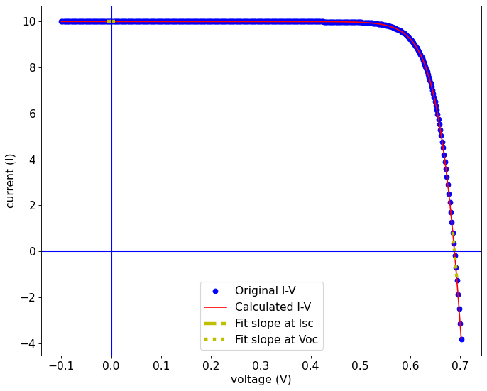
As you can see, the I-V curve parameters extraction method is accurate provided that the slopes at Voc and Isc are well defined.

data_size = 50
I_noise = 0
IV_curve = model_IV(Isc, I0, n, Rs, Rp, temperature, I_noise, data_size)

IL_extr, I0_extr, n_extr, Rs_extr, Rp_extr, slopeFitIsc, slopeFitVoc = get_IV_params(IV_curve, temperature)

IV_curve_extracted = model_IV(IL_extr, I0_extr, n_extr, Rs_extr, Rp_extr, temperature, 0, 500)

# Print the results and errors
print("Rp = " + f"{Rp_extr:.3f}")
#print("Error Rp = " + f"{100*(Rp_extr-Rp)/Rp:.3f}" + " %")
print("Rs = " + f"{Rs_extr:.3e}")
#print("Error Rs = " + f"{100*(Rs_extr-Rs)/Rs:.3f}" + " %")
print("I0 = " + f"{I0_extr:.3}") 
#print("Error I0 = " + f"{100*(I0_extr-I0)/I0:.3f}" + " %")
print("n = " + f"{n_extr:.3f}")
#print("Error n = " + f"{100*(n_extr-n)/n:.3f}" + " %")
print("IL = " + f"{IL_extr:.3f}")
#print("Error Isc = " + f"{100*(Isc_extr-Isc)/Isc:.3f}" + " %")

# Plot the I-V curves
plt.figure(figsize=(10, 8),dpi=80)
plt.plot(IV_curve[:,0], IV_curve[:,1], 'bo', label="Original I-V")
plt.plot(IV_curve_extracted[:,0], IV_curve_extracted[:,1], color='r', label = "Calculated I-V")
plt.plot(slopeFitIsc[:,0],slopeFitIsc[:,1], '--', linewidth=4, color='y', label = "Fit slope at Isc")
plt.plot(slopeFitVoc[:,0],slopeFitVoc[:,1], ':', linewidth=4, color='y', label = "Fit slope at Voc")
#plt.ylim((-0.01, Isc*1.1))
plt. axvline(x=0,linewidth=1, color='b')
plt. axhline(y=0,linewidth=1, color='b')
plt.xlabel('voltage (V)', size=14)
plt.ylabel('current (I)', size=14)
plt.xticks(fontsize=14)
plt.yticks(fontsize=14)
plt.legend(fontsize=14)
plt.show()

Rp = 499.959
Rs = 1.789e-03
I0 = 1.89e-10
n = 1.084
IL = 10.000

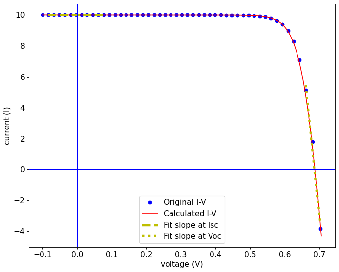
For a low number of datapoints, the resolution around Voc is low and the calculation of the slope is not accurate enough. The I-V curve parameters extracted can present a significant error.

data_size = 100
I_noise = 0.02
IV_curve = model_IV(Isc, I0, n, Rs, Rp, temperature, I_noise, data_size)

IL_extr, I0_extr, n_extr, Rs_extr, Rp_extr, slopeFitIsc, slopeFitVoc = get_IV_params(IV_curve, temperature)

IV_curve_extracted = model_IV(IL_extr, I0_extr, n_extr, Rs_extr, Rp_extr, temperature, 0, 500)

# Print the results and errors
print("Rp = " + f"{Rp_extr:.3f}")
#print("Error Rp = " + f"{100*(Rp_extr-Rp)/Rp:.3f}" + " %")
print("Rs = " + f"{Rs_extr:.3e}")
#print("Error Rs = " + f"{100*(Rs_extr-Rs)/Rs:.3f}" + " %")
print("I0 = " + f"{I0_extr:.3}") 
#print("Error I0 = " + f"{100*(I0_extr-I0)/I0:.3f}" + " %")
print("n = " + f"{n_extr:.3f}")
#print("Error n = " + f"{100*(n_extr-n)/n:.3f}" + " %")
print("IL = " + f"{IL_extr:.3f}")
#print("Error Isc = " + f"{100*(Isc_extr-Isc)/Isc:.3f}" + " %")

# Plot the I-V curves
plt.figure(figsize=(10, 8),dpi=80)
plt.plot(IV_curve[:,0], IV_curve[:,1], 'bo', label="Original I-V")
plt.plot(IV_curve_extracted[:,0], IV_curve_extracted[:,1], color='r', label = "Calculated I-V")
plt.plot(slopeFitIsc[:,0],slopeFitIsc[:,1], '--', linewidth=4, color='y', label = "Fit slope at Isc")
plt.plot(slopeFitVoc[:,0],slopeFitVoc[:,1], ':', linewidth=4, color='y', label = "Fit slope at Voc")
#plt.ylim((-0.01, Isc*1.1))
plt. axvline(x=0,linewidth=1, color='b')
plt. axhline(y=0,linewidth=1, color='b')
plt.xlabel('voltage (V)', size=14)
plt.ylabel('current (I)', size=14)
plt.xticks(fontsize=14)
plt.yticks(fontsize=14)
plt.legend(fontsize=14)
plt.show()

Rp = -0.670
Rs = -3.101e-04
I0 = 1.77e-05
n = 2.006
IL = 10.108

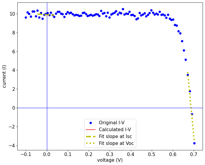
When the number of datapoints is too low or there is significant noise in the data, these slopes can be difficult to obtain from an I-V curve, giving poor fitting results.
You can try to improve the algorithm by, for example, changing the number of datapoints where the slopes are evaluated. This is useful if the total number of datapoints can´t be too high because of technical restrictions (for example if the I-V curve measurement can´t last too long)
You can also take a larger range of voltages around V=0 to fit the I-V curve and calculate the slope. This way the noise can be averaged and its effect reduced.