
Problem 12.5#
Fundamentals of Solar Cells and Photovoltaic Systems Engineering
Solutions Manual - Chapter 12
Problem 12.5
The tabulated data provided in the online repository of this book includes hourly irradiance data for the different solar irradiance components measured in Madrid, Spain, on June 10 at a fixed plane at a tilt of 35⁰, which is very close to the optimum inclination (for maximum energy capture throughout the year) at such latitude.
(a) For every hour, estimate the diffuse irradiance from the global and direct components and compare them to the experimentally measured diffuse irradiance. Calculate the root-mean-square error (RMSE) between both time series.
(b) What are the typical instruments used to obtain such experimental data?
We will use the package pandas to handle the data and matplotlib.pyplot to plot the results.
import pandas as pd
import numpy as np
import matplotlib.pyplot as plt
We start by importing the measured solar irradiance components.
G = pd.read_csv('data/Global_35deg.csv', index_col=0, header=0)
B = pd.read_csv('data/Direct_35deg.csv', index_col=0, header=0)
D = pd.read_csv('data/Diffuse_35deg.csv', index_col=0, header=0)
B
| Gb(i) | |
|---|---|
| time(UTC+1) | |
| 00:00 | 0.00 |
| 01:00 | 0.00 |
| 02:00 | 0.00 |
| 03:00 | 0.00 |
| 04:00 | 0.00 |
| 05:00 | 0.00 |
| 06:00 | 0.00 |
| 07:00 | 5.90 |
| 08:00 | 131.87 |
| 09:00 | 291.56 |
| 10:00 | 439.15 |
| 11:00 | 569.09 |
| 12:00 | 633.52 |
| 13:00 | 653.63 |
| 14:00 | 610.45 |
| 15:00 | 533.22 |
| 16:00 | 423.96 |
| 17:00 | 286.50 |
| 18:00 | 140.95 |
| 19:00 | 21.13 |
| 20:00 | 0.00 |
| 21:00 | 0.00 |
| 22:00 | 0.00 |
| 23:00 | 0.00 |
We can estimated the diffuse irradiance \(D\) by substracting the direct irradiance \(B\) from the global irradiance \(G\).
D_estimated = G['G(i)']-B['Gb(i)']
D_estimated
time(UTC+1)
00:00      0.00
01:00      0.00
02:00      0.00
03:00      0.00
04:00      0.00
05:00      0.00
06:00     13.34
07:00     57.23
08:00    106.95
09:00    147.89
10:00    183.18
11:00    206.35
12:00    233.26
13:00    244.38
14:00    244.52
15:00    234.24
16:00    211.69
17:00    172.14
18:00    124.94
19:00     69.31
20:00     24.39
21:00      0.00
22:00      0.00
23:00      0.00
dtype: float64
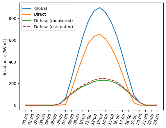
We can plot the measured and estimated irradiance components.
plt.plot(G['G(i)'],
         linewidth=2, label='Global')
plt.plot(B['Gb(i)'],
         linewidth=2, label='Direct')
plt.plot(D['Gd(i)'],
         linewidth=2, label='Diffuse (measured)')
plt.plot(D_estimated,
         linewidth=2, linestyle='--',label='Diffuse (estimated)')
plt.ylabel('Irradiance (W/m2)')
plt.xticks(rotation=70)
plt.legend()
<matplotlib.legend.Legend at 0x7f19ba0a0e50>
We calculate the root-mean square error (RMSE) between the estimated and measured diffuse irradiance.
RMSE=np.sqrt(((D['Gd(i)']-D_estimated)**2).mean())
print('The RMSE is ' + str(RMSE.round(2)) + ' W/m2')
The RMSE is 8.41 W/m2
(b) What are the typical instruments used to obtain such experimental data?
Global irradiance is measured using a pyranometer. Direct irradiance using a pyrheliometer. Diffuse irradiance can be measured using a pyranometer together with an element to block direct irradiance.