Problem 15.7

Fundamentals of Solar Cells and Photovoltaic Systems Engineering

Solutions Manual - Chapter 15

Problem 15.7

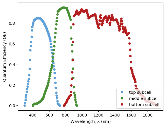
Figure 15.9 shows the Quantum Efficiency (QE) of a space triple junction solar cell at BOL. The tabulated data is available in the online repository of this book. Check if the total current and the top/mid current balance under the AM0 spectrum are better than the result obtained in Problem 15.6.

We will use the package pandas to handle the data and matplotlib.pyplot to plot the results.

import pandas as pd
import numpy as np
import matplotlib.pyplot as plt

We start by importing the data for the solar spectra.

datafile = pd.read_csv('data/Reference_spectrum_ASTM-G173-03.csv', index_col=0, header=0) 
datafile

	AM0	AM1.5G	AM1.5D
Wvlgth nm	Etr W*m-2*nm-1	Global tilt W*m-2*nm-1	Direct+circumsolar W*m-2*nm-1
280	8.20E-02	4.73E-23	2.54E-26
280.5	9.90E-02	1.23E-21	1.09E-24
281	1.50E-01	5.69E-21	6.13E-24
281.5	2.12E-01	1.57E-19	2.75E-22
...	...	...	...
3980	8.84E-03	7.39E-03	7.40E-03
3985	8.80E-03	7.43E-03	7.45E-03
3990	8.78E-03	7.37E-03	7.39E-03
3995	8.70E-03	7.21E-03	7.23E-03
4000	8.68E-03	7.10E-03	7.12E-03

2003 rows × 3 columns

datafile.drop(datafile.index[0], inplace=True)   #remove row including information on units
datafile=datafile.astype(float)                  #convert values to float for easy operation
datafile.index=datafile.index.astype(float)      #convert indexes to float for easy operation

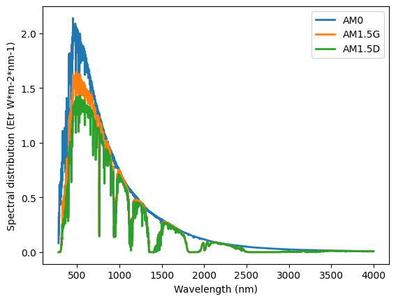
We can also plot the three spectra

plt.plot(datafile, 
         linewidth=2, label=datafile.columns)
plt.ylabel('Spectral distribution (Etr W*m-2*nm-1)')
plt.xlabel('Wavelength (nm)')
plt.legend()

<matplotlib.legend.Legend at 0x7fc72ad47d50>

We define the relevant constants and import the QE of the triple junction solar cell.

h=6.63*10**(-34)   # [J·s] Planck constant
e=1.60*10**(-19)   # [C] electron charge
c =299792458       #[m/s] Light speed

QE_top = pd.read_csv('data/EQE_TC_BOL.txt', 
                     header=None, index_col=0, sep='\t').dropna().squeeze() #import dataframe and convert into series
QE_mid = pd.read_csv('data/EQE_MC_BOL.txt', 
                     header=None, index_col=0, sep='\t').squeeze() #import dataframe and convert into series 
QE_bot = pd.read_csv('data/EQE_BC_BOL.txt', 
                     header=None, index_col=0, sep='\t').squeeze() #import dataframe and convert into series 

We can plot the Quantum Efficiency.

plt.plot(QE_top, linewidth=0, label='top subcell', marker='.', markersize=10, color='#5FA1D8') #ligthblue
plt.plot(QE_mid, linewidth=0, label='middle subcell', marker='.', markersize=10, color='#498F34') #green
plt.plot(QE_bot, linewidth=0, label='bottom subcell', marker='.', markersize=10, color='#B31F20') #darkred
plt.ylabel('Quantum Efficiency (QE)')
plt.xlabel('Wavelength, $\lambda$ (nm)');
plt.legend(loc='lower right')

<matplotlib.legend.Legend at 0x7fc727709f90>

For the top subcell, we calculate the spectral response, interpolate the spectrum, and integrate to obtain the short-circuit current density using Eq. 3.5.

\(J=\int SR(\lambda) \cdot G(\lambda) \ d\lambda\)

In this case, we assume the extraterrestrial irradiance AM0.

QE=QE_top
SR=pd.Series(index=QE.index,
            data=[QE.loc[i]*e*i*0.000000001/(h*c) for i in QE.index])

spectrum='AM0'
spectra=datafile[spectrum]
spectra_interpolated=np.interp(SR.index, spectra.index, spectra.values)

J_top = np.trapz([x*y for x,y in zip(SR, spectra_interpolated)], x=SR.index)*1000/10000 # A-> mA ; m2 -> cm2
print('Photocurrent density top = ' + str(J_top.round(1)) + ' mA/cm2')

Photocurrent density top = 16.4 mA/cm2

We repeat the analysis for the middle subcell.

QE=QE_mid
SR=pd.Series(index=QE.index,
            data=[QE.loc[i]*e*i*0.000000001/(h*c) for i in QE.index])

spectra=datafile[spectrum]
spectra_interpolated=np.interp(SR.index, spectra.index, spectra.values)

J_mid = np.trapz([x*y for x,y in zip(SR, spectra_interpolated)], x=SR.index)*1000/10000 # A-> mA ; m2 -> cm2
print('Photocurrent density middle = ' + str(J_mid.round(1)) + ' mA/cm2')

Photocurrent density middle = 18.2 mA/cm2

We repeat the analysis for the bottom subcell.

QE=QE_bot
SR=pd.Series(index=QE.index,
            data=[QE.loc[i]*e*i*0.000000001/(h*c) for i in QE.index])

spectra=datafile[spectrum]
spectra_interpolated=np.interp(SR.index, spectra.index, spectra.values)

J_bot = np.trapz([x*y for x,y in zip(SR, spectra_interpolated)], x=SR.index)*1000/10000 # A-> mA ; m2 -> cm2
print('Photocurrent density bottom = ' + str(J_bot.round(1)) + ' mA/cm2')

Photocurrent density bottom = 29.7 mA/cm2

The current balance of the top and middle subcells (\(J_{SC,top}\)/\(J_{SC,middle}\)) can be calculated as follows:

J_top/J_mid

0.9026416870694149

In this case, the top subcell is limiting the current flowing through the device since it produces 10% less current than the middle subcell. We can say that here the match is better because the current produced by the top and mid subcell is more similar than in Problem 15.6.