Problem 3.6

Fundamentals of Solar Cells and Photovoltaic Systems Engineering

Solutions Manual - Chapter 3

Problem 3.6

Using the standard tabulated data (file “Reference_spectrum_ASTM-G173-03.csv” in the online repository of the book):

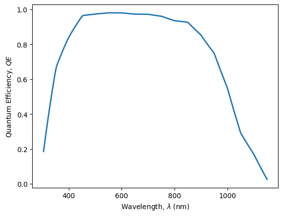
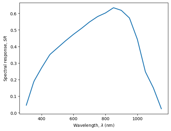
Using the provided Quantum Efficiency (QE), calculate the Spectral Response (SR) of a Silicon solar cell. Plot the QE and SR as a function of wavelength

(b) Estimate the photocurrent density generated by a silicon solar cell illuminated by the reference spectrum AM1.5G.

We will use the package pandas to handle the data and matplotlib.pyplot to plot the results

import pandas as pd
import numpy as np
import matplotlib.pyplot as plt

We start by importing the data.

datafile = pd.read_csv('data/Reference_spectrum_ASTM-G173-03.csv', index_col=0, header=0) 
datafile

	AM0	AM1.5G	AM1.5D
Wvlgth nm	Etr W*m-2*nm-1	Global tilt W*m-2*nm-1	Direct+circumsolar W*m-2*nm-1
280	8.20E-02	4.73E-23	2.54E-26
280.5	9.90E-02	1.23E-21	1.09E-24
281	1.50E-01	5.69E-21	6.13E-24
281.5	2.12E-01	1.57E-19	2.75E-22
...	...	...	...
3980	8.84E-03	7.39E-03	7.40E-03
3985	8.80E-03	7.43E-03	7.45E-03
3990	8.78E-03	7.37E-03	7.39E-03
3995	8.70E-03	7.21E-03	7.23E-03
4000	8.68E-03	7.10E-03	7.12E-03

2003 rows × 3 columns

datafile.drop(datafile.index[0], inplace=True) #remove row including information on units
datafile=datafile.astype(float) #convert values to float for easy operation
datafile.index=datafile.index.astype(float) #convert indexes to float for easy operation

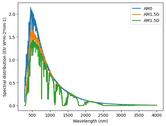
We can plot the spectra.

plt.plot(datafile, linewidth=2, label=datafile.columns)
plt.ylabel('Spectral distribution (Etr W*m-2*nm-1)')
plt.xlabel('Wavelength (nm)')
plt.legend()

<matplotlib.legend.Legend at 0x7f847159cb10>

We define the relevant constants.

h=6.63*10**(-34) # [J·s] Planck constant
e=1.60*10**(-19) #C electron charge
c =299792458 #[m/s] Light speed

QE = pd.read_csv('data/QE_Silicon.csv', index_col=0, header=0) 
QE

	QE Silicon Solar cell
nm
305	0.185579
310	0.243200
315	0.298992
320	0.353041
325	0.405425
...	...
1130	0.081951
1135	0.067769
1140	0.053712
1145	0.039777
1150	0.025964

170 rows × 1 columns

We plot the Quantum Efficiency and Spectral Response

SR=pd.Series(index=QE.index,
            data=[QE.loc[i,'QE Silicon Solar cell']*e*i*0.000000001/(h*c) for i in QE.index])
SR

nm
305     0.045563
310     0.060689
315     0.075815
320     0.090941
325     0.106067
          ...   
1130    0.074545
1135    0.061918
1140    0.049290
1145    0.036663
1150    0.024036
Length: 170, dtype: float64

plt.plot(QE, 
         linewidth=2)
plt.ylabel('Quantum Efficiency, $QE$')
plt.xlabel('Wavelength, $\lambda$ (nm)');

plt.plot(SR, 
         linewidth=2)
plt.ylabel('Spectral response, $SR$')
plt.xlabel(r'Wavelength, $\lambda$ (nm)');

(c) Estimate the photocurrent generated by a Silicon solar cell illuminated by the reference spectrum AM1.5 G

First, we need to interpolate the spectra at those datapoints included in the SR.

spectra=datafile['AM1.5G']
spectra_interpolated=np.interp(SR.index, spectra.index, spectra.values)

Then, we calculate the photocurrent using Eq. 3.5.

\(J=\int SR(\lambda) \cdot G(\lambda) \ d\lambda\)

J = np.trapz([x*y for x,y in zip(SR, spectra_interpolated)], x=SR.index)*1000/10000 # A-> mA ; m2 -> cm2
print('Photocurrent density = ' + str(J.round(1)) + ' mA/cm2')

Photocurrent density = 36.7 mA/cm2