Problem 12.1

Fundamentals of Solar Cells and Photovoltaic Systems Engineering

Solutions Manual - Chapter 12

Problem 12.1

In this problem, we will review the method to extract the main parameters in the I-V curve presented in Chapter 4. Let us assume that we have measured the dark I-V curve of a 10 cm\(^2\) solar cell at 25 \(^{\circ}\)C. The tabulated data is provided in this book’s online repository. The series resistance \(R_s\) can be assumed to be zero so the dark I-V curve equation is:

\(I = I_0(e^{(qV/nkT)}-1)+ \frac{V}{R_p}\)

Estimate the reverse saturation current \(I_0\), the diode ideality factor \(n\), and discuss the potential effect of the parallel resistance \(R_p\).

We will use the package pandas to handle the data and matplotlib.pyplot to plot the results.

import pandas as pd
import numpy as np
import matplotlib.pyplot as plt
import math

We start by importing the data from the dark I-V curves.

dark_IV = pd.read_csv('data/Dark_I_V_curve.csv',  header=0) 
dark_IV.head()

	V (V)	I (A)
0	0.1598	0.000003
1	0.2239	0.000004
2	0.2657	0.000006
3	0.3099	0.000008
4	0.3568	0.000011

Following the strategy described in the Advanced Materials of Chapter 4 (Dark I-V curve of solar cells), we plot the curve using a log y-axis.

plt.plot(dark_IV['V (V)'], dark_IV['I (A)'],
         linewidth=2, marker='o', markerfacecolor="None",
         label='dark')
plt.yscale('log')
plt.ylabel('Current (A)')
plt.xlabel('Voltage (V)')
plt.xlim([0,1])


#fit the dark IV curve plotted with a log y-axis
value_at_0V=5*10**-9
slope=18.5
plt.plot(np.append(0, dark_IV['V (V)'].values), 
         [math.exp(math.log(value_at_0V)+slope*V) for V in np.append(0, dark_IV['V (V)'].values)],
         linewidth=2, linestyle='--',color='firebrick',
         label='fitting')
plt.legend()

<matplotlib.legend.Legend at 0x7fa59096a250>

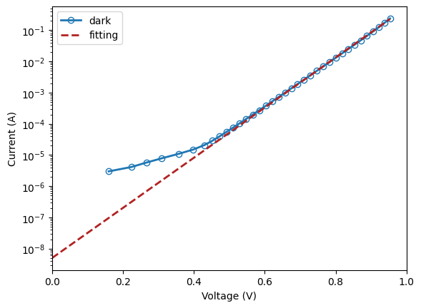
We have also plotted the linear fit to the dark IV curve ploted using a log y axis. The slope of the curve allow us the calculate the ideality coefficient.

\(ln(I)=ln(I_0)+ \frac{V}{nKT/q}\)

#assuming that the measuremen was taking at 25C
KT_q=0.025

n=1/(slope*KT_q)
print("n = " + str(round(n,2)))

n = 2.16

The value of the fit at 0V indicates the reverse saturation current

I_0=value_at_0V
print("I_0 = " + str(I_0))

I_0 = 5e-09

The deviation of the IV curve from the linear fitting (in log-y representation) for high voltage values represents the effect of series resistance \(R_s\). In this case, the fitting is almost perfect, indicating that there is no significant \(R_s\).

The deviation of the IV curve from the linear fitting (in log-y representation) for low volage values represents the effect of parallel resistance \(R_p\). In this case, the curve deviates from the linear fitting but only at current values below \(10^{-4}\). As discussed in the Advanced Materials of Chapter 4, this should not create any significant reduction in the cell FF or efficiency.