Problem 12.2

Fundamentals of Solar Cells and Photovoltaic Systems Engineering

Solutions Manual - Chapter 12

Problem 12.2

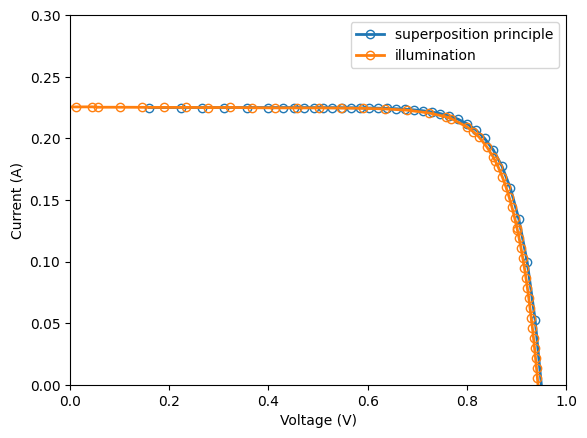
Assume that, in addition to the dark I-V curve provided in the previous problem, we have also measured the I-V curve under illumination. The latter has been measured under standard test conditions (STC), that is 1000 W/m\(^2\) and AM1.5G spectrum, and is provided in this book online repository. You are asked to verify the superposition principle between the dark I-V curve and the illumination I-V curve, described in Chapter 4. To that end, add a photogenerated current \(I_L\) to the dark I-V curve and compare it with the experimental I-V curve under illumination Estimate the \(I_L\) value that results in the best fitting of both curves. Take into account that the dark or recombination current and the photogenerated current have opposite signs.

We will use the package pandas to handle the data and matplotlib.pyplot to plot the results.

import pandas as pd
import numpy as np
import matplotlib.pyplot as plt

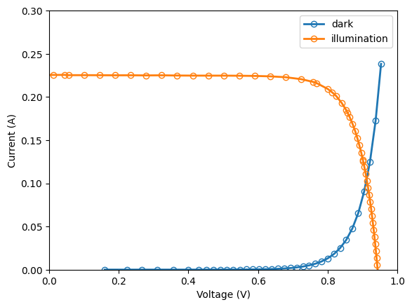
We start by importing the data from the dark and illumination I-V curves.

dark_IV = pd.read_csv('data/Dark_I_V_curve.csv',  header=0) 
dark_IV.head()

	V (V)	I (A)
0	0.1598	0.000003
1	0.2239	0.000004
2	0.2657	0.000006
3	0.3099	0.000008
4	0.3568	0.000011

illum_IV = pd.read_csv('data/Illumination_I_V_curve.csv',  header=0) 
illum_IV.head()

	V (V)	I (A)
0	-0.3000	0.226923
1	-0.2555	0.226572
2	-0.2110	0.226254
3	-0.1665	0.225777
4	-0.1219	0.225872

We can plot both curves.

plt.plot(dark_IV['V (V)'], dark_IV['I (A)'],
         linewidth=2, marker='o', markerfacecolor="None",
         label='dark')
plt.plot(illum_IV['V (V)'], illum_IV['I (A)'],
         linewidth=2, marker='o',markerfacecolor="None",
         label='illumination')
plt.ylabel('Current (A)')
plt.xlabel('Voltage (V)')
plt.xlim([0,1])
plt.ylim([0,0.3])
plt.legend()

<matplotlib.legend.Legend at 0x7f89d41adc90>

We can try different values of photogenerated current \(I_L\), apply the superposition principle, and plot the measured IV curve under illumination and the estimated IV curve. Visually, we can select the \(I_L\) that maximizes the fitting between both curves.

I_L=0.225
superposed_IV = dark_IV.copy()
superposed_IV['I (A)'] = I_L - dark_IV['I (A)']

plt.plot(superposed_IV['V (V)'], superposed_IV['I (A)'],
         linewidth=2, marker='o', markerfacecolor="None",
         label='superposition principle')
plt.plot(illum_IV['V (V)'], illum_IV['I (A)'],
         linewidth=2, marker='o', markerfacecolor="None",
         label='illumination')
plt.ylabel('Current (A)')
plt.xlabel('Voltage (V)')
plt.xlim([0,1])
plt.ylim([0,0.3])
plt.legend()

<matplotlib.legend.Legend at 0x7f89d3f077d0>