Introduction to numpy

Introduction to `numpy`#

Note

This material is mostly adapted from the following resources:

Numpy is the fundamental package for scientific computing with Python. NumPy is the standard Python library used for working with arrays (i.e., vectors & matrices), linear algebra, and other numerical computations.

Website: https://numpy.org/
GitHub: numpy/numpy

Note

Documentation for this package is available at https://numpy.org/doc/stable/index.html.

Note

If you have not yet set up Python on your computer, you can execute this tutorial in your browser via Google Colab. Click on the rocket in the top right corner and launch “Colab”. If that doesn’t work download the .ipynb file and import it in Google Colab

Then install numpy by executing the following command in a Jupyter cell at the top of the notebook.

!pip install numpy

Importing a Package#

This will be our first experience with importing a package.

Usually we import numpy with the alias np.

import numpy as np

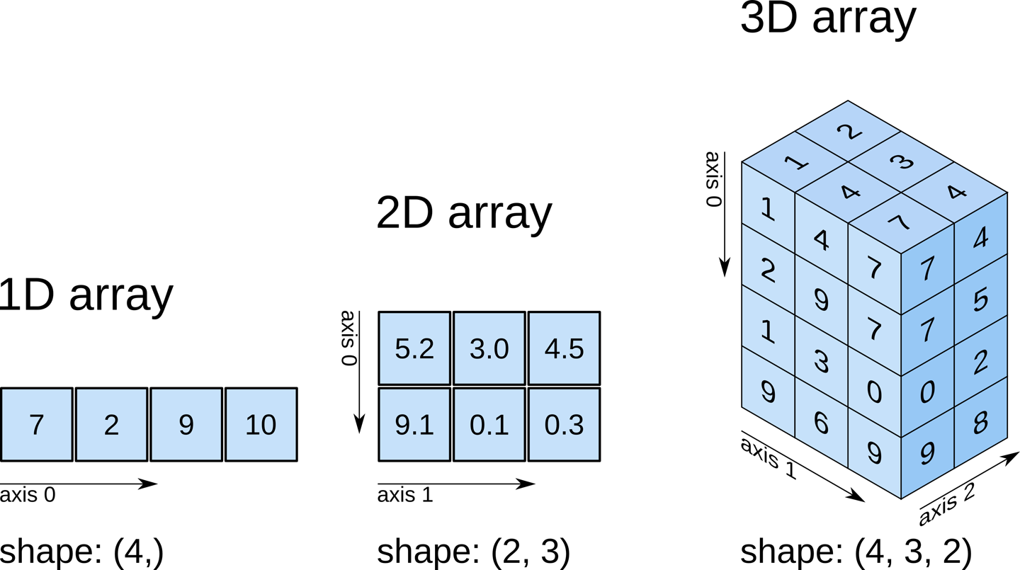
NDArrays#

NDarrays (short for n-dimensional arrays) are a key data structure in numpy. NDarrays are similar to Python lists, but they allow fast, efficient computations on large arrays and matrices of numerical data. NDarrays can have any number of dimensions, and are used for a wide range of numerical and scientific computing tasks, including linear algebra, statistical analysis, and image processing.

Thus, the main differences between a numpy array and a list are the following:

numpy arrays can have N dimensions (while lists only have 1)
numpy arrays hold values of the same datatype (e.g. int, float), while lists can contain anything.
numpy optimizes numerical operations on arrays. Numpy is fast!

# create an array from a list
a = np.array([9, 0, 2, 1, 0])

Note

If you’re in Jupyter, you can use <shift> + <tab> to inspect a function.

# find out the datatype
a.dtype

dtype('int64')

# find out the shape
a.shape

(5,)

# another array with a different datatype and shape
b = np.array([[5, 3, 1, 9], [9, 2, 3, 0]], dtype=np.float64)

# check dtype
b.dtype

dtype('float64')

# check shape
b.shape

(2, 4)

Array Creation#

There are lots of ways to create arrays.

np.zeros((4, 4))

array([[0., 0., 0., 0.],
       [0., 0., 0., 0.],
       [0., 0., 0., 0.],
       [0., 0., 0., 0.]])

np.ones((2, 2, 3))

array([[[1., 1., 1.],
        [1., 1., 1.]],

       [[1., 1., 1.],
        [1., 1., 1.]]])

np.full((3, 2), np.pi)

array([[3.14159265, 3.14159265],
       [3.14159265, 3.14159265],
       [3.14159265, 3.14159265]])

np.random.rand(5, 2)

array([[0.94486309, 0.43520131],
       [0.02294564, 0.63665755],
       [0.16668522, 0.74535374],
       [0.93606162, 0.52278158],
       [0.60372367, 0.17603061]])

np.arange(10)

array([0, 1, 2, 3, 4, 5, 6, 7, 8, 9])

np.arange(2, 4, 0.25)

array([2.  , 2.25, 2.5 , 2.75, 3.  , 3.25, 3.5 , 3.75])

A frequent need is to generate an array of N numbers, evenly spaced between two values. That is what linspace is for.

np.linspace(2, 4, 20)

array([2.        , 2.10526316, 2.21052632, 2.31578947, 2.42105263,
       2.52631579, 2.63157895, 2.73684211, 2.84210526, 2.94736842,
       3.05263158, 3.15789474, 3.26315789, 3.36842105, 3.47368421,
       3.57894737, 3.68421053, 3.78947368, 3.89473684, 4.        ])

Numpy also has some utilities for helping us generate multi-dimensional arrays. For instance, meshgrid creates 2D arrays out of a combination of 1D arrays.

x = np.linspace(-2 * np.pi, 2 * np.pi, 5)
y = np.linspace(-np.pi, np.pi, 4)
xx, yy = np.meshgrid(x, y)
xx.shape, yy.shape

((4, 5), (4, 5))

yy

array([[-3.14159265, -3.14159265, -3.14159265, -3.14159265, -3.14159265],
       [-1.04719755, -1.04719755, -1.04719755, -1.04719755, -1.04719755],
       [ 1.04719755,  1.04719755,  1.04719755,  1.04719755,  1.04719755],
       [ 3.14159265,  3.14159265,  3.14159265,  3.14159265,  3.14159265]])

xx

array([[-6.28318531, -3.14159265,  0.        ,  3.14159265,  6.28318531],
       [-6.28318531, -3.14159265,  0.        ,  3.14159265,  6.28318531],
       [-6.28318531, -3.14159265,  0.        ,  3.14159265,  6.28318531],
       [-6.28318531, -3.14159265,  0.        ,  3.14159265,  6.28318531]])

Indexing#

Basic indexing in numpy is similar to lists.

# get some individual elements of xx
xx[3, 4]

6.283185307179586

# get some whole rows
xx[0]

array([-6.28318531, -3.14159265,  0.        ,  3.14159265,  6.28318531])

# get some whole columns
xx[:, -1]

array([6.28318531, 6.28318531, 6.28318531, 6.28318531])

# get some ranges (also called slicing)
xx[0:2, 3:5]

array([[3.14159265, 6.28318531],
       [3.14159265, 6.28318531]])

Broadcasting#

Not all the arrays we want to work with will have the same size!

Broadcasting is a powerful feature in numpy that allows you to perform operations on arrays of different shapes and sizes. It automatically expands the smaller array to match the dimensions of the larger array, without actually making copies of the data, so that element-wise operations can be performed. This is done by following a set of rules that determine how the shapes of the arrays align.

Broadcasting allows you to vectorize operations and avoid explicit loops, leading to more concise and efficient code. It’s particularly useful when working with large data sets, as it helps optimize memory usage and computational speed.

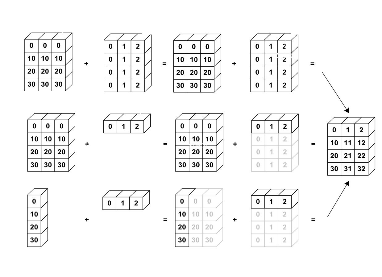
Dimensions are automatically aligned starting with the last dimension. If the last two dimensions have the same length, then the two arrays can be broadcast.

f = np.sin(xx) * np.cos(0.5 * yy)
print(f.shape, x.shape)

(4, 5) (5,)

g = f * x

print(g.shape)

(4, 5)

Reduction Operations#

In data science, we usually start with a lot of data and want to reduce it down in order to make plots of summary tables.

There are many different reduction operations. The table below lists the most common functions:

Reduction Operation	Description
`numpy.sum()`	Computes the sum of array elements over a given axis.
`numpy.mean()`	Computes the arithmetic mean along a specified axis.
`numpy.min()`	Computes the minimum value along a specified axis.
`numpy.max()`	Computes the maximum value along a specified axis.
`numpy.prod()`	Computes the product of array elements over a given axis.
`numpy.std()`	Computes the standard deviation along a specified axis.
`numpy.var()`	Computes the variance along a specified axis.

# sum
g.sum()

-3.9982744542688894e-15

# mean
g.mean()

-1.9991372271344446e-16

# standard deviation
g.std()

5.809358098232775e-16

A key property of numpy reductions is the ability to operate on just one axis.

# apply on just one axis
g_ymean = g.mean(axis=0)
g_xmean = g.mean(axis=1)

Exercises#

Import numpy under the alias np.

Create the following arrays:

Create an array of 5 zeros.
Create an array of 10 ones.
Create an array of 5 \(\pi\) values.
Create an array of the integers 1 to 20.
Create a 5 x 5 matrix of ones with a dtype int.

Create a 3D matrix of 3 x 3 x 3 full of random numbers drawn from a standard normal distribution (hint: np.random.randn())

Create an array of 20 linearly spaced numbers between 1 and 10.

Below I’ve defined an array of shape 4 x 4. Use indexing to produce the given outputs.

array([[ 9, 10],
       [14, 15],
       [19, 20],
       [24, 25]])

array([ 6,  7,  8,  9, 10])

array([[11, 12, 13, 14, 15],
       [16, 17, 18, 19, 20]])

array([[ 8,  9],
       [13, 14]])

Calculate the sum of all the numbers in a.

Calculate the sum of each row in a.

Extract all values of a greater than the mean of a (hint: use a boolean mask).

Introduction to numpy

Contents

Introduction to numpy#

Importing a Package#

NDArrays#

Array Creation#

Indexing#

Broadcasting#

Reduction Operations#

Exercises#

Introduction to `numpy`#