Introduction to pvlib#
pvlib is a set of documented functions for simulating the performance of photovoltaic energy systems.
GitHub: pvlib/pvlib-python
Documentation for this package is available at https://pvlib-python.readthedocs.io/en/stable/. You can also check out the pvlib python examples gallery
You can ask for help and find useful discussion on the pvlib-python Google Group
Note
If you have not yet set up Python on your computer, you can execute this tutorial in your browser via Google Colab. Click on the rocket in the top right corner and launch “Colab”. If that doesn’t work download the .ipynb file and import it in Google Colab.
Then install pandas and numpy by executing the following command in a Jupyter cell at the top of the notebook.
!pip install pandas numpy pvlib
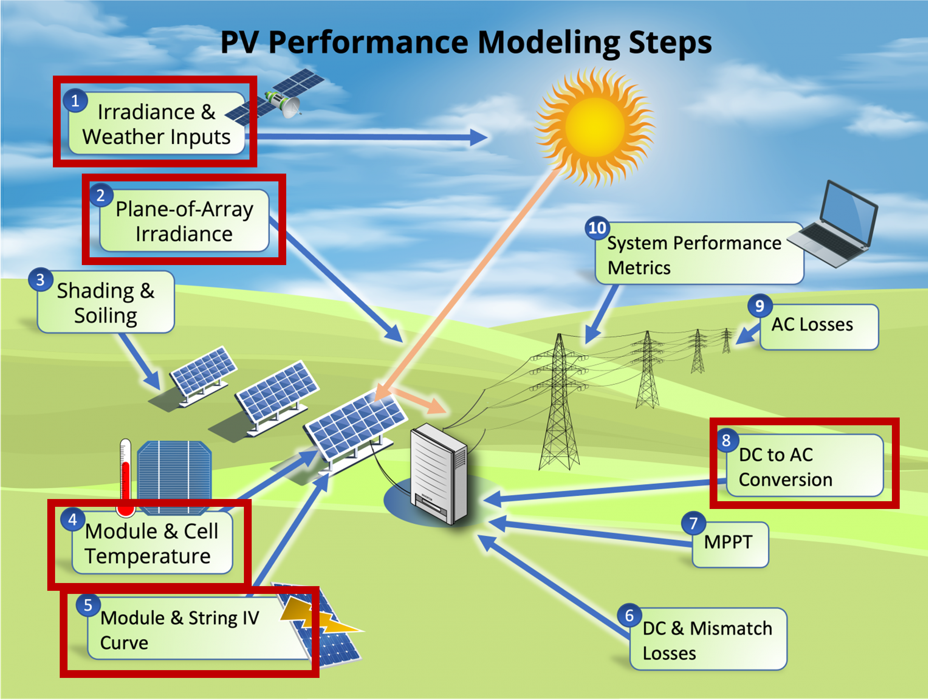
The sketch below from the Sandia PV Performance Modeling Collaborative (PVPMC) outlines the topics covered in this introduction:
1 - Access weather data (e.g. typical meteorological year -TMY-), understand solar irradiance data, and visualize it.#
Typical Meteorological Year (TMY) datasets are intended to represent the weather for a typical year at a given location.
TMY datasets provide hourly solar irradiance, air temperature, wind speed, and other weather measurements for a hypothetical year that represents more or less a “median year” for solar resource.
We start importing the packages that we will use.
import os  # for getting environment variables
import pathlib  # for finding the example dataset
import pvlib
import pandas as pd
import matplotlib.pyplot as plt
Reading a TMY dataset with pvlib
First, we’ll read the TMY dataset with pvlib.iotools.read_tmy3() which returns a Pandas DataFrame of the timeseries weather data and a second output with a Python dictionary of the TMY metadata like longitude, latitude, elevation, etc.
We will use the Python pathlib to get the path to the 'data' directory which comes with the pvlib package. Then we can use the slash operator, / to make the full path to the TMY file.
help(pvlib.iotools.read_tmy3)
Help on function read_tmy3 in module pvlib.iotools.tmy:

read_tmy3(filename, coerce_year=None, map_variables=True, encoding=None)
    Read a TMY3 file into a pandas dataframe.

    Note that values contained in the metadata dictionary are unchanged
    from the TMY3 file (i.e. units are retained). In the case of any
    discrepancies between this documentation and the TMY3 User's Manual
    [1]_, the TMY3 User's Manual takes precedence.

    The TMY3 files were updated in Jan. 2015. This function requires the
    use of the updated files.

    Parameters
    ----------
    filename : str
        A relative file path or absolute file path.
    coerce_year : int, optional
        If supplied, the year of the index will be set to ``coerce_year``, except
        for the last index value which will be set to the *next* year so that
        the index increases monotonically.
    map_variables : bool, default True
        When True, renames columns of the DataFrame to pvlib variable names
        where applicable. See variable :const:`VARIABLE_MAP`.
    encoding : str, optional
        Encoding of the file. For files that contain non-UTF8 characters it may
        be necessary to specify an alternative encoding, e.g., for
        SolarAnywhere TMY3 files the encoding should be 'iso-8859-1'. Users
        may also consider using the 'utf-8-sig' encoding.

    Returns
    -------
    Tuple of the form (data, metadata).

    data : DataFrame
        A pandas dataframe with the columns described in the table
        below. For more detailed descriptions of each component, please
        consult the TMY3 User's Manual [1]_, especially tables 1-1
        through 1-6.

    metadata : dict
        The site metadata available in the file.

    Notes
    -----
    The returned structures have the following fields.

    ===============   ======  ===================
    key               format  description
    ===============   ======  ===================
    altitude          Float   site elevation
    latitude          Float   site latitudeitude
    longitude         Float   site longitudeitude
    Name              String  site name
    State             String  state
    TZ                Float   UTC offset
    USAF              Int     USAF identifier
    ===============   ======  ===================


    ========================       ======================================================================================================================================================
    field                          description
    ========================       ======================================================================================================================================================
    **† denotes variables that are mapped when `map_variables` is True**
    -------------------------------------------------------------------------------------------------------------------------------------------------------------------------------------
    Index                          A pandas datetime index. NOTE, the index is timezone aware, and times are set to local standard time (daylight savings is not included)
    ghi_extra†                     Extraterrestrial horizontal radiation recv'd during 60 minutes prior to timestamp, Wh/m^2
    dni_extra†                     Extraterrestrial normal radiation recv'd during 60 minutes prior to timestamp, Wh/m^2
    ghi†                           Direct and diffuse horizontal radiation recv'd during 60 minutes prior to timestamp, Wh/m^2
    GHI source                     See [1]_, Table 1-4
    GHI uncert (%)                 Uncertainty based on random and bias error estimates see [2]_
    dni†                           Amount of direct normal radiation (modeled) recv'd during 60 mintues prior to timestamp, Wh/m^2
    DNI source                     See [1]_, Table 1-4
    DNI uncert (%)                 Uncertainty based on random and bias error estimates see [2]_
    dhi†                           Amount of diffuse horizontal radiation recv'd during 60 minutes prior to timestamp, Wh/m^2
    DHI source                     See [1]_, Table 1-4
    DHI uncert (%)                 Uncertainty based on random and bias error estimates see [2]_
    GH illum (lx)                  Avg. total horizontal illuminance recv'd during the 60 minutes prior to timestamp, lx
    GH illum source                See [1]_, Table 1-4
    GH illum uncert (%)            Uncertainty based on random and bias error estimates see [2]_
    DN illum (lx)                  Avg. direct normal illuminance recv'd during the 60 minutes prior to timestamp, lx
    DN illum source                See [1]_, Table 1-4
    DN illum uncert (%)            Uncertainty based on random and bias error estimates see [2]_
    DH illum (lx)                  Avg. horizontal diffuse illuminance recv'd during the 60 minutes prior to timestamp, lx
    DH illum source                See [1]_, Table 1-4
    DH illum uncert (%)            Uncertainty based on random and bias error estimates see [2]_
    Zenith lum (cd/m^2)            Avg. luminance at the sky's zenith during the 60 minutes prior to timestamp, cd/m^2
    Zenith lum source              See [1]_, Table 1-4
    Zenith lum uncert (%)          Uncertainty based on random and bias error estimates see [1]_ section 2.10
    TotCld (tenths)                Amount of sky dome covered by clouds or obscuring phenonema at time stamp, tenths of sky
    TotCld source                  See [1]_, Table 1-5
    TotCld uncert (code)           See [1]_, Table 1-6
    OpqCld (tenths)                Amount of sky dome covered by clouds or obscuring phenonema that prevent observing the sky at time stamp, tenths of sky
    OpqCld source                  See [1]_, Table 1-5
    OpqCld uncert (code)           See [1]_, Table 1-6
    temp_air†                      Dry bulb temperature at the time indicated, deg C
    Dry-bulb source                See [1]_, Table 1-5
    Dry-bulb uncert (code)         See [1]_, Table 1-6
    temp_dew†                      Dew-point temperature at the time indicated, deg C
    Dew-point source               See [1]_, Table 1-5
    Dew-point uncert (code)        See [1]_, Table 1-6
    relative_humidity†             Relatitudeive humidity at the time indicated, percent
    RHum source                    See [1]_, Table 1-5
    RHum uncert (code)             See [1]_, Table 1-6
    pressure†                      Station pressure at the time indicated, 1 mbar
    Pressure source                See [1]_, Table 1-5
    Pressure uncert (code)         See [1]_, Table 1-6
    wind_direction†                Wind direction at time indicated, degrees from north (360 = north; 0 = undefined,calm)
    Wdir source                    See [1]_, Table 1-5
    Wdir uncert (code)             See [1]_, Table 1-6
    wind_speed†                    Wind speed at the time indicated, meter/second
    Wspd source                    See [1]_, Table 1-5
    Wspd uncert (code)             See [1]_, Table 1-6
    Hvis (m)                       Distance to discernable remote objects at time indicated (7777=unlimited), meter
    Hvis source                    See [1]_, Table 1-5
    Hvis uncert (coe)              See [1]_, Table 1-6
    CeilHgt (m)                    Height of cloud base above local terrain (7777=unlimited), meter
    CeilHgt source                 See [1]_, Table 1-5
    CeilHgt uncert (code)          See [1]_, Table 1-6
    precipitable_water†            Total precipitable water contained in a column of unit cross section from earth to top of atmosphere, cm
    Pwat source                    See [1]_, Table 1-5
    Pwat uncert (code)             See [1]_, Table 1-6
    AOD                            The broadband aerosol optical depth per unit of air mass due to extinction by aerosol component of atmosphere, unitless
    AOD source                     See [1]_, Table 1-5
    AOD uncert (code)              See [1]_, Table 1-6
    albedo†                        The ratio of reflected solar irradiance to global horizontal irradiance, unitless
    Alb source                     See [1]_, Table 1-5
    Alb uncert (code)              See [1]_, Table 1-6
    Lprecip depth (mm)             The amount of liquid precipitation observed at indicated time for the period indicated in the liquid precipitation quantity field, millimeter
    Lprecip quantity (hr)          The period of accumulatitudeion for the liquid precipitation depth field, hour
    Lprecip source                 See [1]_, Table 1-5
    Lprecip uncert (code)          See [1]_, Table 1-6
    PresWth (METAR code)           Present weather code, see [2]_.
    PresWth source                 Present weather code source, see [2]_.
    PresWth uncert (code)          Present weather code uncertainty, see [2]_.
    ========================       ======================================================================================================================================================

    .. admonition:: Midnight representation

       The function is able to handle midnight represented as 24:00 (NREL TMY3
       format, see [1]_) and as 00:00 (SolarAnywhere TMY3 format, see [3]_).

    .. warning:: TMY3 irradiance data corresponds to the *previous* hour, so
        the first index is 1AM, corresponding to the irradiance from midnight
        to 1AM, and the last index is midnight of the *next* year. For example,
        if the last index in the TMY3 file was 1988-12-31 24:00:00 this becomes
        1989-01-01 00:00:00 after calling :func:`~pvlib.iotools.read_tmy3`.

    .. warning:: When coercing the year, the last index in the dataframe will
        become midnight of the *next* year. For example, if the last index in
        the TMY3 was 1988-12-31 24:00:00, and year is coerced to 1990 then this
        becomes 1991-01-01 00:00:00.

    References
    ----------
    .. [1] Wilcox, S and Marion, W. "Users Manual for TMY3 Data Sets".
       NREL/TP-581-43156, Revised May 2008.
       :doi:`10.2172/928611`
    .. [2] Wilcox, S. (2007). National Solar Radiation Database 1991 2005
       Update: Users Manual. 472 pp.; NREL Report No. TP-581-41364.
       :doi:`10.2172/901864`
    .. [3] `SolarAnywhere file formats
       <https://www.solaranywhere.com/support/historical-data/file-formats/>`_
DATA_DIR = pathlib.Path(pvlib.__file__).parent / 'data'
df_tmy, metadata = pvlib.iotools.read_tmy3(DATA_DIR / '723170TYA.CSV',
                                            coerce_year=1990,
                                           map_variables=True)
metadata  # display the dictionary of metadata
{'USAF': 723170,
 'Name': '"GREENSBORO PIEDMONT TRIAD INT"',
 'State': 'NC',
 'TZ': -5.0,
 'latitude': 36.1,
 'longitude': -79.95,
 'altitude': 273.0}
Let’s display the first 4 lines of the dataframe
df_tmy.head(4)
| Date (MM/DD/YYYY) | Time (HH:MM) | ghi_extra | dni_extra | ghi | GHI source | GHI uncert (%) | dni | DNI source | DNI uncert (%) | ... | albedo | Alb source | Alb uncert (code) | Lprecip depth (mm) | Lprecip quantity (hr) | Lprecip source | Lprecip uncert (code) | PresWth (METAR code) | PresWth source | PresWth uncert (code) | |
|---|---|---|---|---|---|---|---|---|---|---|---|---|---|---|---|---|---|---|---|---|---|
| 1990-01-01 01:00:00-05:00 | 01/01/1988 | 01:00 | 0 | 0 | 0 | 1 | 0 | 0 | 1 | 0 | ... | 0.0 | ? | 0 | 0 | 1 | D | 9 | 0 | C | 8 |
| 1990-01-01 02:00:00-05:00 | 01/01/1988 | 02:00 | 0 | 0 | 0 | 1 | 0 | 0 | 1 | 0 | ... | 0.0 | ? | 0 | 0 | 1 | D | 9 | 0 | C | 8 |
| 1990-01-01 03:00:00-05:00 | 01/01/1988 | 03:00 | 0 | 0 | 0 | 1 | 0 | 0 | 1 | 0 | ... | 0.0 | ? | 0 | 0 | 1 | D | 9 | 0 | C | 8 |
| 1990-01-01 04:00:00-05:00 | 01/01/1988 | 04:00 | 0 | 0 | 0 | 1 | 0 | 0 | 1 | 0 | ... | 0.0 | ? | 0 | 0 | 1 | D | 9 | 0 | C | 8 |
4 rows × 71 columns
This dataset follows the standard format of handling timeseries data with pandas – one row per timestamp, one column per measurement type. Because TMY files represent one year of data (no leap years), that means they’ll have 8760 rows. The number of columns can vary depending on the source of the data.
print("Number of rows:", len(df_tmy))
print("Number of columns:", len(df_tmy.columns))
Number of rows: 8760
Number of columns: 71
You can access single rows by pointing to its number location (iloc) or by using the index name it has. In this case, the index is a dateTime
df_tmy.iloc[0]
Date (MM/DD/YYYY)        01/01/1988
Time (HH:MM)                  01:00
ghi_extra                         0
dni_extra                         0
ghi                               0
                            ...
Lprecip source                    D
Lprecip uncert (code)             9
PresWth (METAR code)              0
PresWth source                    C
PresWth uncert (code)             8
Name: 1990-01-01 01:00:00-05:00, Length: 71, dtype: object
df_tmy.loc['1990-01-01 01:00:00-05:00']
Date (MM/DD/YYYY)        01/01/1988
Time (HH:MM)                  01:00
ghi_extra                         0
dni_extra                         0
ghi                               0
                            ...
Lprecip source                    D
Lprecip uncert (code)             9
PresWth (METAR code)              0
PresWth source                    C
PresWth uncert (code)             8
Name: 1990-01-01 01:00:00-05:00, Length: 71, dtype: object
You can also print all the column names in the dataframe
df_tmy.keys()
Index(['Date (MM/DD/YYYY)', 'Time (HH:MM)', 'ghi_extra', 'dni_extra', 'ghi',
       'GHI source', 'GHI uncert (%)', 'dni', 'DNI source', 'DNI uncert (%)',
       'dhi', 'DHI source', 'DHI uncert (%)', 'GH illum (lx)',
       'GH illum source', 'Global illum uncert (%)', 'DN illum (lx)',
       'DN illum source', 'DN illum uncert (%)', 'DH illum (lx)',
       'DH illum source', 'DH illum uncert (%)', 'Zenith lum (cd/m^2)',
       'Zenith lum source', 'Zenith lum uncert (%)', 'TotCld (tenths)',
       'TotCld source', 'TotCld uncert (code)', 'OpqCld (tenths)',
       'OpqCld source', 'OpqCld uncert (code)', 'temp_air', 'Dry-bulb source',
       'Dry-bulb uncert (code)', 'temp_dew', 'Dew-point source',
       'Dew-point uncert (code)', 'relative_humidity', 'RHum source',
       'RHum uncert (code)', 'pressure', 'Pressure source',
       'Pressure uncert (code)', 'wind_direction', 'Wdir source',
       'Wdir uncert (code)', 'wind_speed', 'Wspd source', 'Wspd uncert (code)',
       'Hvis (m)', 'Hvis source', 'Hvis uncert (code)', 'CeilHgt (m)',
       'CeilHgt source', 'CeilHgt uncert (code)', 'precipitable_water',
       'Pwat source', 'Pwat uncert (code)', 'AOD (unitless)', 'AOD source',
       'AOD uncert (code)', 'albedo', 'Alb source', 'Alb uncert (code)',
       'Lprecip depth (mm)', 'Lprecip quantity (hr)', 'Lprecip source',
       'Lprecip uncert (code)', 'PresWth (METAR code)', 'PresWth source',
       'PresWth uncert (code)'],
      dtype='object')
There are 71 columns, which is quite a lot! For now, let’s focus just on the ones that are most important for PV modeling – the irradiance, temperature, and wind speed columns, and extract them into a new DataFrame.
For this NREL TMY3 dataset the units of irradiance are W/m², air temperature is in °C, and wind speed is m/s.
# GHI, DHI, DNI are irradiance measurements
# DryBulb is the "dry-bulb" (ambient) temperature
# Wspd is wind speed
df = df_tmy[['ghi', 'dhi', 'dni', 'temp_air', 'wind_speed']]
# show the first 15 rows:
df.head(15)
| ghi | dhi | dni | temp_air | wind_speed | |
|---|---|---|---|---|---|
| 1990-01-01 01:00:00-05:00 | 0 | 0 | 0 | 10.0 | 6.2 |
| 1990-01-01 02:00:00-05:00 | 0 | 0 | 0 | 10.0 | 5.2 |
| 1990-01-01 03:00:00-05:00 | 0 | 0 | 0 | 10.0 | 5.7 |
| 1990-01-01 04:00:00-05:00 | 0 | 0 | 0 | 10.0 | 5.7 |
| 1990-01-01 05:00:00-05:00 | 0 | 0 | 0 | 10.0 | 5.2 |
| 1990-01-01 06:00:00-05:00 | 0 | 0 | 0 | 10.0 | 4.1 |
| 1990-01-01 07:00:00-05:00 | 0 | 0 | 0 | 10.0 | 4.1 |
| 1990-01-01 08:00:00-05:00 | 9 | 9 | 1 | 10.0 | 5.2 |
| 1990-01-01 09:00:00-05:00 | 46 | 46 | 3 | 10.0 | 5.2 |
| 1990-01-01 10:00:00-05:00 | 79 | 78 | 4 | 10.6 | 5.2 |
| 1990-01-01 11:00:00-05:00 | 199 | 198 | 3 | 11.7 | 6.2 |
| 1990-01-01 12:00:00-05:00 | 261 | 260 | 3 | 11.7 | 5.2 |
| 1990-01-01 13:00:00-05:00 | 155 | 155 | 0 | 11.7 | 5.2 |
| 1990-01-01 14:00:00-05:00 | 144 | 144 | 2 | 11.7 | 3.1 |
| 1990-01-01 15:00:00-05:00 | 131 | 131 | 1 | 11.1 | 4.1 |
Plotting time series data with pandas and matplotlib
Let’s make some plots to get a better idea of what TMY data gives us.
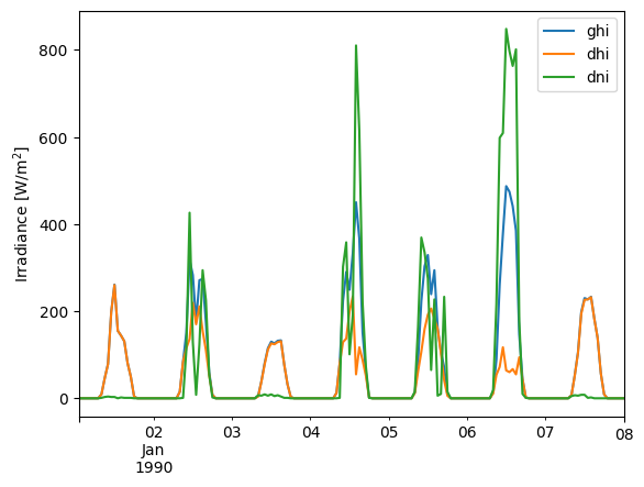
First, the three irradiance fields:
first_week = df.head(24*7)  # Plotting 7 days, each one has 24 hours or entries
first_week[['ghi', 'dhi', 'dni']].plot()
plt.ylabel('Irradiance [W/m$^2$]');
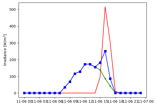
Let’s control the parameters a bit more
birthday = df.loc['1990-11-06':'1990-11-06']
plt.plot(birthday['dni'], color='r')
plt.plot(birthday['dhi'], color='g', marker='.')
plt.plot(birthday['ghi'], color='b', marker='s')
plt.ylabel('Irradiance [W/m$^2$]');
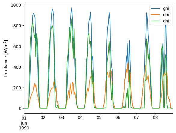
We can also plot a summer week.
summer_week = df.loc['1990-06-01':'1990-06-08']
summer_week[['ghi', 'dhi', 'dni']].plot()
plt.ylabel('Irradiance [W/m$^2$]');
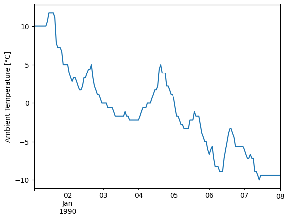
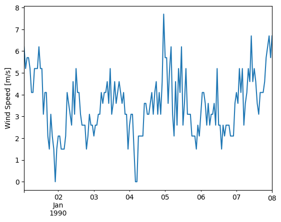
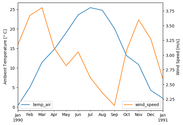
We can also plot the air temperature and wind speed.
first_week['temp_air'].plot()
plt.ylabel('Ambient Temperature [°C]');
first_week['wind_speed'].plot()
plt.ylabel('Wind Speed [m/s]');
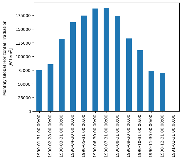
Pandas makes it easy to roll-up timeseries data into summary values. We can use the DataFrame.resample() function with DateOffsets like 'M' for months. For example, we can calculate total monthly GHI as a quick way to visualize the seasonality of solar resource:
# summing hourly irradiance (W/m^2) gives insolation (W h/m^2)
monthly_ghi = df['ghi'].resample('M').sum()
monthly_ghi.head(4)
/tmp/ipykernel_3886/44194593.py:2: FutureWarning: 'M' is deprecated and will be removed in a future version, please use 'ME' instead.
  monthly_ghi = df['ghi'].resample('M').sum()
1990-01-31 00:00:00-05:00     74848
1990-02-28 00:00:00-05:00     85751
1990-03-31 00:00:00-05:00    131766
1990-04-30 00:00:00-05:00    162302
Freq: ME, Name: ghi, dtype: int64
monthly_ghi = monthly_ghi.tz_localize(None)  # don't need timezone for monthly data
monthly_ghi.plot.bar()
plt.ylabel('Monthly Global Horizontal Irradiation \n[W h/m$^2$]');
We can also take monthly averages instead of monthly sums:
fig, ax1 = plt.subplots()
ax2 = ax1.twinx()  # add a second y-axis
monthly_average_temp_wind = df[['temp_air', 'wind_speed']].resample('M').mean()
monthly_average_temp_wind['temp_air'].plot(ax=ax1, c='tab:blue')
monthly_average_temp_wind['wind_speed'].plot(ax=ax2, c='tab:orange')
ax1.set_ylabel(r'Ambient Temperature [$\degree$ C]')
ax2.set_ylabel(r'Wind Speed [m/s]')
ax1.legend(loc='lower left')
ax2.legend(loc='lower right');
/tmp/ipykernel_3886/4038915213.py:3: FutureWarning: 'M' is deprecated and will be removed in a future version, please use 'ME' instead.
  monthly_average_temp_wind = df[['temp_air', 'wind_speed']].resample('M').mean()
2. Calculate plane of array (POA) irradiance#
The amount of sunlight collected by a PV panel depends on how well the panel orientation matches incoming sunlight. The three components of solar irradiance must be tansposed on the plane of array (POA) and added to calculate the total POA irradiance.
How is array orientation defined?
Two parameters define the panel orientation, one that measures the cardinal direction (North, East, South, West), and one that measures how high in the sky the panel faces:
tilt; measured in degrees from horizontal. A flat panel is at tilt=0 and a panel standing on its edge has tilt=90.
azimuth; measured in degrees from North. The direction along the horizon the panel is facing. N=0, E=90, S=180, W=270.
A fixed array has fixed tilt and azimuth, but a tracker array constantly changes its orientation to best match the sun’s position. So depending on the system configuration, tilt and azimuth may or may not be time series values.
# First, let's make a Location object corresponding to the TMY that we have previously imported
location = pvlib.location.Location(latitude=metadata['latitude'],
                                   longitude=metadata['longitude'])
Because part of the transposition process requires knowing where the sun is in the sky, let’s use pvlib to calculate solar position. TMY data represents the average weather conditions across each hour, meaning we need to calculate solar position in the middle of each hour. pvlib calculates solar position for the exact timestamps you specify, so we need to adjust the times by half an interval (30 minutes):
# Note: TMY datasets are right-labeled hourly intervals, e.g. the
# 10AM to 11AM interval is labeled 11.  We should calculate solar position in
# the middle of the interval (10:30), so we subtract 30 minutes:
times = df_tmy.index - pd.Timedelta('30min')
solar_position = location.get_solarposition(times)
# but remember to shift the index back to line up with the TMY data:
solar_position.index += pd.Timedelta('30min')

solar_position.head()
| apparent_zenith | zenith | apparent_elevation | elevation | azimuth | equation_of_time | |
|---|---|---|---|---|---|---|
| 1990-01-01 01:00:00-05:00 | 166.841893 | 166.841893 | -76.841893 | -76.841893 | 6.889661 | -3.395097 |
| 1990-01-01 02:00:00-05:00 | 160.512529 | 160.512529 | -70.512529 | -70.512529 | 52.424214 | -3.414863 |
| 1990-01-01 03:00:00-05:00 | 149.674856 | 149.674856 | -59.674856 | -59.674856 | 73.251821 | -3.434619 |
| 1990-01-01 04:00:00-05:00 | 137.777090 | 137.777090 | -47.777090 | -47.777090 | 85.208599 | -3.454365 |
| 1990-01-01 05:00:00-05:00 | 125.672180 | 125.672180 | -35.672180 | -35.672180 | 94.134730 | -3.474102 |
The two values needed here are the solar zenith (how close the sun is to overhead) and azimuth (what direction along the horizon the sun is, like panel azimuth). The difference between apparent_zenith and zenith is that apparent_zenith includes the effect of atmospheric refraction.
Now that we have a time series of solar position that matches our irradiance data, let’s run a transposition model using the convenient wrapper function pvlib.irradiance.get_total_irradiance. The more complex transposition models like Perez and Hay Davies require additional weather inputs, so for simplicity we’ll just use the basic isotropic model here, which is the default if nothing is passed for model keyword argument. As an example, we’ll model a fixed array tilted south at 20 degrees.
df_poa = pvlib.irradiance.get_total_irradiance(
        surface_tilt=20,  # tilted 20 degrees from horizontal
        surface_azimuth=180,  # facing South
        dni=df_tmy['dni'],
        ghi=df_tmy['ghi'],
        dhi=df_tmy['dhi'],
        solar_zenith=solar_position['apparent_zenith'],
        solar_azimuth=solar_position['azimuth'],
        model='isotropic')
get_total_irradiance returns a DataFrame containing each of the POA components mentioned earlier (direct, diffuse, and ground), along with the total in-plane irradiance.
df_poa.keys()
Index(['poa_global', 'poa_direct', 'poa_diffuse', 'poa_sky_diffuse',
       'poa_ground_diffuse'],
      dtype='object')
Let’s visualize monthly global radiation to summarize the difference between the irradiation received by a flat panel (GHI) and that of a tilted panel (POA):
df = pd.DataFrame({
    'ghi': df_tmy['ghi'],
    'poa': df_poa['poa_global'],
})
df_monthly = df.resample('M').sum()
df_monthly.plot.bar()
plt.ylabel('Monthly irradiation [W h/m$^2$]');
/tmp/ipykernel_3886/3845930564.py:5: FutureWarning: 'M' is deprecated and will be removed in a future version, please use 'ME' instead.
  df_monthly = df.resample('M').sum()
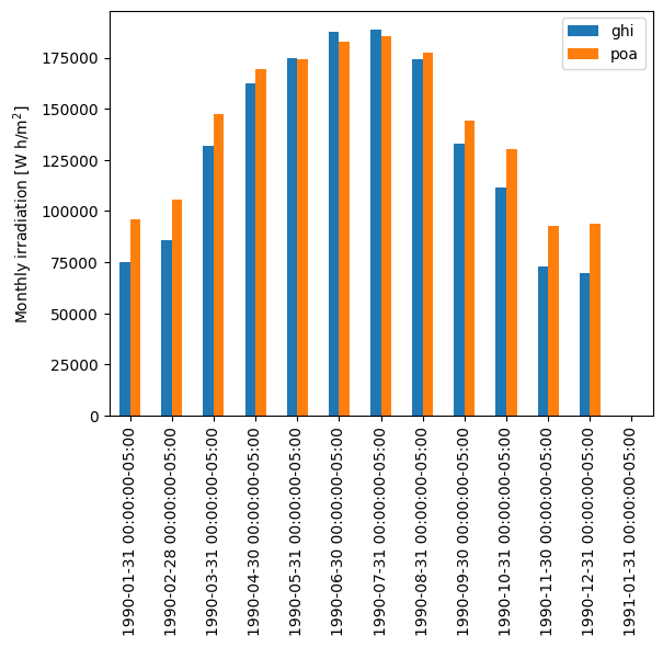
This plot shows that, compared with a flat array, a tilted array receives significantly more irradiation in the winter. However, it comes at the cost of slightly less irradiation in the summer.
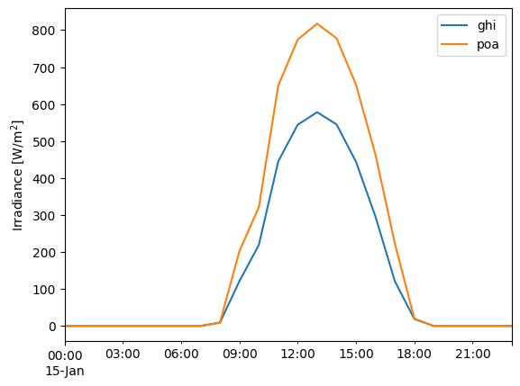
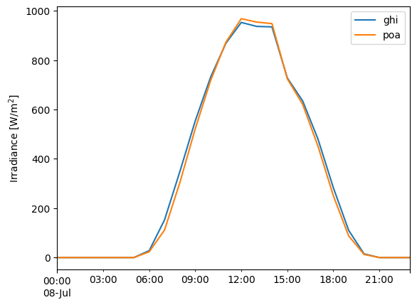
Let’s look at a sunny day in winter vs a sunny day in summer.
df.loc['1990-01-15'].plot()
plt.ylabel('Irradiance [W/m$^2$]');
df.loc['1990-07-08'].plot()
plt.ylabel('Irradiance [W/m$^2$]');
Modeling POA for a tracking system
The previous section calculated the transposition assuming a fixed array tilt and azimuth. Now we’ll do the same for a tracking array that follows the sun across the sky. The most common type of tracking array is what’s called a horizonalsingle-axis tracker (HSAT) that rotates from East to West to follow the sun. We can calculate the time-dependent orientation of a HSAT array with pvlib:
tracker_data = pvlib.tracking.singleaxis(
                solar_position['apparent_zenith'],
                solar_position['azimuth'],
            axis_azimuth=180,  # axis is aligned N-S
            )  # leave the rest of the singleaxis parameters like backtrack and gcr at their defaults
tilt = tracker_data['surface_tilt'].fillna(0)
azimuth = tracker_data['surface_azimuth'].fillna(0)

# plot a day to illustrate:
tracker_data['tracker_theta'].fillna(0).head(24).plot()
plt.ylabel('Tracker Rotation [degrees]');
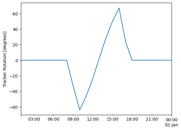
This plot shows a single day of tracker operation. The y-axis shows the tracker rotation from horizontal, so 0 degrees means the panels are flat. In the morning, the trackers rotate to negative angles to face East towards the morning sun; in the afternoon they rotate to positive angles to face West towards the evening sun. In the middle of the day, the trackers are flat because the sun is more or less overhead.
Now we can model the irradiance collected by a tracking array – we follow the same procedure as before, but using the timeseries tilt and azimuth this time:
df_poa_tracker = pvlib.irradiance.get_total_irradiance(
    surface_tilt=tilt,  # time series for tracking array
    surface_azimuth=azimuth,  # time series for tracking array
    dni=df_tmy['dni'],
    ghi=df_tmy['ghi'],
    dhi=df_tmy['dhi'],
    solar_zenith=solar_position['apparent_zenith'],
    solar_azimuth=solar_position['azimuth'])
tracker_poa = df_poa_tracker['poa_global']
df.loc['1990-01-15', 'ghi'].plot()
tracker_poa.loc['1990-01-15'].plot()
plt.legend()
plt.ylabel('Irradiance [W/m$^2$]');
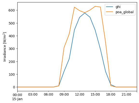
The tracking system can tilt the array steeply East and West to face towards the sun in early morning and late afternoon, meaning the edges of day get much higher irradiance than for a south-facing array.
Note that the POA calculations discussed above do not address the partial blocking of diffuse light in arrays with multiple tilted rows of PV modules, so the results will be slightly (typically 1-3%) optimistic relative to real conditions or to commercial modeling software.
3. Calculate module temperature from ambient data.#
Here we will use the thermal model from the Sandia Array Performance Model (SAPM) to estimate cell temperature from ambient conditions. The SAPM thermal model takes only POA irradiance, ambient temperature, and wind speed as weather inputs, but it also requires a set of parameters that characterize the thermal properties of the module of interest as the module’s mounting configuration. Parameter values covering the common system designs are provided with pvlib:
all_parameters = pvlib.temperature.TEMPERATURE_MODEL_PARAMETERS['sapm']
list(all_parameters.keys())
['open_rack_glass_glass',
 'close_mount_glass_glass',
 'open_rack_glass_polymer',
 'insulated_back_glass_polymer']
open_rack_glass_polymer is appropriate for many large-scale systems (polymer backsheet; open racking), so we will use it here:
parameters = all_parameters['open_rack_glass_polymer']
# note the "splat" operator "**" which expands the dictionary "parameters"
# into a comma separated list of keyword arguments
cell_temperature = pvlib.temperature.sapm_cell(
    tracker_poa, df_tmy['temp_air'], df_tmy['wind_speed'], **parameters)
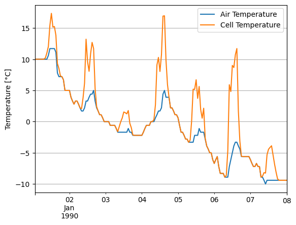
Let’s compare ambient temperature with cell temperature. Notice how our modeled cell temperature rises significantly above ambient temperature during the day, especially on sunny days:
df_tmy['temp_air'].head(24*7).plot()
cell_temperature.head(24*7).plot()
plt.grid()
plt.legend(['Air Temperature', 'Cell Temperature'])
plt.ylabel('Temperature [°C]');
Wind speed also has an effect, but it’s harder to see in a time series plot like this. To make it clearer, let’s make a scatter plot:
temperature_difference = cell_temperature - df_tmy['temp_air']
plt.scatter(tracker_poa, temperature_difference, c=df_tmy['wind_speed'])
plt.colorbar()
plt.ylabel('Temperature rise above ambient [$\degree C$]')
plt.xlabel('POA Irradiance [$W/m^2$]');
plt.title('Cell temperature rise, colored by wind speed')
Text(0.5, 1.0, 'Cell temperature rise, colored by wind speed')
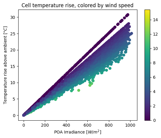
The main trend is a bigger temperature difference as incident irradiance increases. However, this plot shows that higher wind speed reduces the effect – faster wind means more convective cooling, so a lower cell temperature than it would be in calm air.
Note: the gap at the upper edge of the trend is an artifact of the low resolution of wind speed values in this TMY dataset; there are no values between 0 and 0.3 m/s.
4. Use POA irradiance and module temperature to model a PV module’s performance.#
Now that we know how to obtain the plane of array (POA) irradiance and cell temperature, let’s calculate the array’s output power.
Here we will use one of the more basic PV models implemented by pvlib. The PVWatts module model requires only two array parameters – the array size (nameplate capacity) and the array’s efficiency dependence on cell temperature.
For demonstration purposes, we’ll assume a 1 kW array with horizontal single axis tracking (HSAT) and a temperature coefficient of -0.4%/°C:
gamma_pdc = -0.004 # -0.4 %/°C
nameplate = 1e3
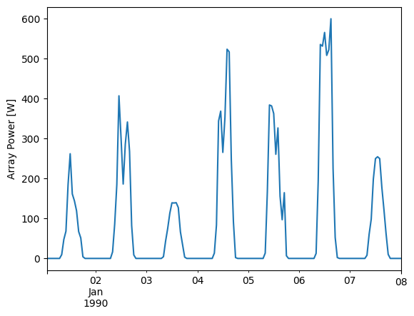
array_power = pvlib.pvsystem.pvwatts_dc(tracker_poa, cell_temperature, nameplate, gamma_pdc)
array_power.head(24*7).plot()
plt.ylabel('Array Power [W]');
Let’s take a look at the array’s response to irradiance and temperature:
plt.scatter(tracker_poa, array_power, c=df_tmy['temp_air'])
plt.colorbar()
plt.ylabel('Array Power [W]')
plt.xlabel('POA Irradiance [W/m^2]')
plt.title('Power vs POA, colored by amb. temp.');
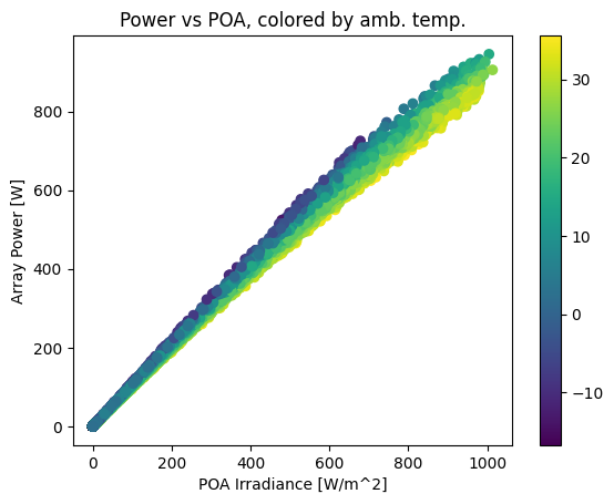
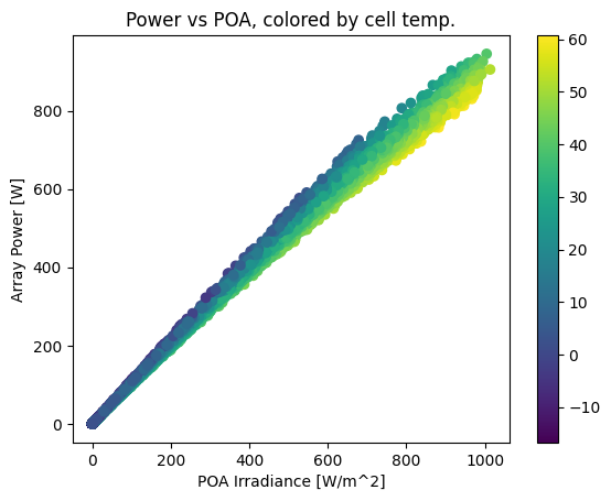
This plot shows a strong, near-linear trend of power with POA irradiance. However, it also shows a performance change with temperature – as ambient temperature increases, array output drops. The gradient is smoother if we color by cell temperature:
plt.scatter(tracker_poa, array_power, c=cell_temperature)
plt.colorbar()
plt.ylabel('Array Power [W]')
plt.xlabel('POA Irradiance [W/m^2]')
plt.title('Power vs POA, colored by cell temp.');
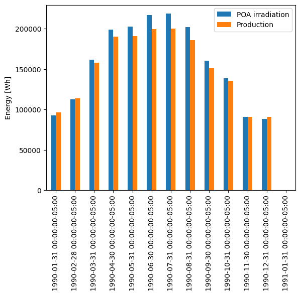
Another way of viewing the temperature effect is to compare monthly energy production with monthly POA irradiation, noticing how production dips relative to irradiation in the summertime. Note that irradiation and production happen to be about the same scale here; that’s just a coincidence because of the array size we chose.
df_plot = pd.DataFrame({
    'POA irradiation': tracker_poa,
    'Production': array_power,
})
# summing hourly power (W) gives (W h)
df_plot.resample('M').sum().plot.bar()
plt.ylabel('Energy [Wh]')
/tmp/ipykernel_3886/3704765181.py:6: FutureWarning: 'M' is deprecated and will be removed in a future version, please use 'ME' instead.
  df_plot.resample('M').sum().plot.bar()
Text(0, 0.5, 'Energy [Wh]')
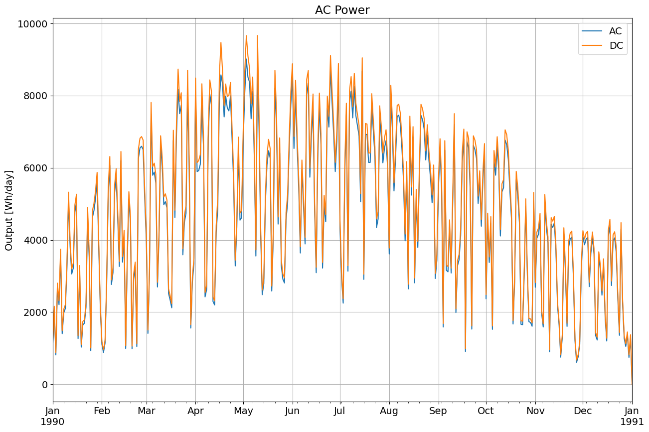
Calculating AC Power
PVWatts has a simplified inverter model. Use pvlib.inverter.pvwatts(pdc, pdc0) to return the AC output given DC output, pdc, and the DC limit, pdc0 which is the AC rated power over the nominal inverter efficiency.
Recall we assumed a 1kW array, so we’ll continue the hypothetical case and assume an AC size of 800W, a DC/AC ratio of 1.2. The default PVWatts nominal inverter efficiency is 0.96 which we use to get pdc0.
pdc0 = 800/0.96  # W
ac = pvlib.inverter.pvwatts(array_power, pdc0)
plt.rcParams['font.size'] = 14
ax = ac.resample('D').sum().plot(figsize=(15, 10), label='AC')
array_power.resample('D').sum().plot(ax=ax, label='DC')
plt.title('AC Power')
plt.ylabel('Output [Wh/day]')
plt.grid()
plt.legend()
<matplotlib.legend.Legend at 0x7f6cc5ae9b50>