Problem 14.7

Fundamentals of Solar Cells and Photovoltaic Systems Engineering

Solutions Manual

Problem 14.7

The objective of this problem is to calculate the local correlation length for wind velocity and solar radiation. We will use the reanalysis dataset ERA5 and weather data corresponding to 2013 that can be downloaded from https://zenodo.org/record/6382570

(a) Select one location in Europe, identify in which grid cell is located and calculate the distance from the other grid cells.

(b) Calculate the Person correlation coefficient from the wind velocity time series and plot the coefficients vs the distance.

(c) Fit the data to an exponential curve and determine the correlation length.

(d) Repeat sections (b) and (c) using the solar irradiation time series.

We will use the packages numpy to operate with arrays and matplotlib.pyplot to plot the results

import numpy as np
import matplotlib.pyplot as  plt
import pandas as pd
import numpy as np
from netCDF4 import Dataset
import geopy.distance

---------------------------------------------------------------------------
ModuleNotFoundError                       Traceback (most recent call last)
Cell In[1], line 6
      4 import numpy as np
      5 from netCDF4 import Dataset
----> 6 import geopy.distance

ModuleNotFoundError: No module named 'geopy'

We load the reanlysis data containing information on wind velocity, solar irradiation, latitude and longitude of the grid cells.

nc = Dataset('../../../../../../Downloads/europe-2013-era5.nc')

We define a data frame that will use to store the calculated results.

data=pd.DataFrame(data=None, 
                  index=None, 
                  columns=['lon', 
                           'lat', 
                           'distance',
                           'rho_wind', 
                           'rho_radiation'], 
                  dtype=float)

As an example, we select Paris. Using the latitude and longitude of this city, the grid cell containing it can be identified.

latitude = 48.86 #Paris
longitude = 2.34
index_lat = np.argmin(np.abs(nc.variables['lat'][:].data-latitude))
index_lon = np.argmin(np.abs(nc.variables['lon'][:].data-longitude))
lon_ref=nc.variables['lon'][index_lon].data
lat_ref=nc.variables['lat'][index_lat].data

The wind velocity and solar radiation in the reference grid cell can be calculated.

wind_ref=nc.variables['wnd100m'][:,index_lat,index_lon].data
radiation_ref = nc.variables['influx_direct'][:,index_lat,index_lon].data+nc.variables['influx_diffuse'][:,index_lat,index_lon].data

For the remaining grid cells, the distance to the reference grid cell, and the correlation coefficient for the wind and solar irradiation time series can be calculated and saved in the data frame. (this can take a few minutes)

To reduce computational time, we select one grid cell every 10 in both latitude and longitud.

i_min=max(0,index_lon-75)
i_max=min(len(nc.variables['lon'][:].data),index_lon+75)
j_min=max(0,index_lat-75)
j_max=min(len(nc.variables['lat'][:].data),index_lat+75)
k=0
for i in np.arange(i_min,i_max, 10):        
    for j in np.arange(j_min,j_max, 10):    
        k=k+1
        lon=nc.variables['lon'][i].data
        data.loc[k, 'lon'] = lon
        
        lat=nc.variables['lat'][j].data
        data.loc[k, 'lat'] = lat

        distance = geopy.distance.geodesic((lat,lon), (lat_ref,lon_ref)).km
        data.loc[k, 'distance'] = distance
        
        wind = nc.variables['wnd100m'][:,j,i]
        radiation = nc.variables['influx_direct'][:,j,i].data+nc.variables['influx_diffuse'][:,j,i].data
        data.loc[k,'rho_wind'] = np.corrcoef(wind,wind_ref)[0,1]
        data.loc[k,'rho_radiation'] = np.corrcoef(radiation,radiation_ref)[0,1]

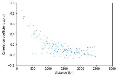
The correlation coefficient for wind time series can be plotted as a function of the distance.

plt.plot(data['distance'],data['rho_wind'],
         marker='.', 
         markersize=2,
         linewidth=0,
         color='dodgerblue')
plt.ylim([-0.2,1])
plt.xlim([0,3000])
plt.ylabel(r'Correlation coefficient $\rho_{g_t^{R_i},g_t^{R_j}}$')
plt.xlabel('distance (km)')

Text(0.5, 0, 'distance (km)')

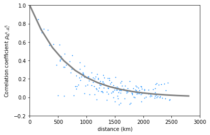
The correlation coefficient can be approach to follow the formula \(\rho_{i,j}=exp(\frac{-1}{\xi_c}·d_{i,j}\)) where \(\xi_c\) is the correlation length. We can check that \(\xi_c\) =650km fits nicely the data points for Paris.

dis=np.arange(0,3000,200)
CL_wind=650
cor_theo_wind=[np.exp(-(1/CL_wind)*d) for d in dis]

plt.plot(data['distance'],data['rho_wind'],
         marker='.', 
         markersize=2,
         linewidth=0,
         color='dodgerblue')
plt.ylim([-0.2,1])
plt.xlim([0,3000])
plt.ylabel(r'Correlation coefficient $\rho_{g_t^{R_i},g_t^{R_j}}$')
plt.xlabel('distance (km)')
plt.plot(dis,cor_theo_wind, 'gray', linewidth=3)

[<matplotlib.lines.Line2D at 0x1f5a53e9608>]

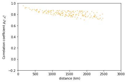
We can plot now the correlation coefficient for solar irradiation and show that the correlation length is much larger in this case.

plt.plot(data['distance'],data['rho_radiation'],
         marker='.', 
         markersize=2,
         linewidth=0,
         color='orange')
plt.ylim([-0.2,1])
plt.xlim([0,3000])
plt.ylabel(r'Correlation coefficient $\rho_{g_t^{R_i},g_t^{R_j}}$')
plt.xlabel('distance (km)')

Text(0.5, 0, 'distance (km)')