
Problem 3.7#
Fundamentals of Solar Cells and Photovoltaic Systems Engineering
Solutions Manual - Chapter 3
Problem 3.7
Let us consider \(P_{max} \approx J_{ideal} · V_{max} · 0.85\) as a rough approximation of the maximum power density produced by an ideal solar cell of bandgap \(E_g\). Here, the factor 0.85 approximates the fill factor, which will be introduced in Chapter 4. \(J_ideal\) is the cell’s ideal photocurrent density (see Box 3.2) and \(V_{max} \approx E_g · 0.75\) (in volts) is an approximated value of the maximum achievable voltage. Calculate the approximate maximum efficiency \(η_{max}\) of a solar cell with a bandgap of 0.2 eV, 0.6 eV, 1.0 eV, 1.4 eV, 1.8 eV, 2.2 eV, and 2.6 eV; when it is illuminated with the reference solar spectrum AM1.5G and discuss the results based on Fig. 3.3.
The spectrum AM1.5G can be found in the file “Reference_spectrum_ASTM-G173-03.csv” in the online repository of the book. The actual solar-cell efficiency limit is described in the Advanced Topic of Chapter 6.
We will use the package pandas to handle the data and matplotlib.pyplot to plot the results
import pandas as pd
import numpy as np
import matplotlib.pyplot as plt
We start by importing the data
datafile = pd.read_csv('data/Reference_spectrum_ASTM-G173-03.csv', index_col=0, header=0)
datafile
| AM0 | AM1.5G | AM1.5D | |
|---|---|---|---|
| Wvlgth nm | Etr W*m-2*nm-1 | Global tilt W*m-2*nm-1 | Direct+circumsolar W*m-2*nm-1 |
| 280 | 8.20E-02 | 4.73E-23 | 2.54E-26 |
| 280.5 | 9.90E-02 | 1.23E-21 | 1.09E-24 |
| 281 | 1.50E-01 | 5.69E-21 | 6.13E-24 |
| 281.5 | 2.12E-01 | 1.57E-19 | 2.75E-22 |
| ... | ... | ... | ... |
| 3980 | 8.84E-03 | 7.39E-03 | 7.40E-03 |
| 3985 | 8.80E-03 | 7.43E-03 | 7.45E-03 |
| 3990 | 8.78E-03 | 7.37E-03 | 7.39E-03 |
| 3995 | 8.70E-03 | 7.21E-03 | 7.23E-03 |
| 4000 | 8.68E-03 | 7.10E-03 | 7.12E-03 |
2003 rows × 3 columns
datafile.drop(datafile.index[0], inplace=True) #remove row including information on units
datafile=datafile.astype(float) #convert values to float for easy operation
datafile.index=datafile.index.astype(float) #convert indexes to float for easy operation
We select the AM1.5G spectrum for our calculations
G = datafile['AM1.5G']
G
280.0     4.730000e-23
280.5     1.230000e-21
281.0     5.690000e-21
281.5     1.570000e-19
282.0     1.190000e-18
              ...
3980.0    7.390000e-03
3985.0    7.430000e-03
3990.0    7.370000e-03
3995.0    7.210000e-03
4000.0    7.100000e-03
Name: AM1.5G, Length: 2002, dtype: float64
We will store all the calculated data in a dataframe
First we define the targeted bandgap values
gaps=np.arange(0.2, 2.7, 0.4)
df = pd.DataFrame()
df['gap eV']=np.round(gaps, 2)
df['gap nm']=np.round(1240/np.array(df['gap eV']),1) #bandgaps in wavelength for esay operation
df=df.set_index('gap eV') #set bandgap in eV as index column
df
| gap nm | |
|---|---|
| gap eV | |
| 0.2 | 6200.0 |
| 0.6 | 2066.7 |
| 1.0 | 1240.0 |
| 1.4 | 885.7 |
| 1.8 | 688.9 |
| 2.2 | 563.6 |
| 2.6 | 476.9 |
For each bandgap, we calculate the maximum voltage
\(V_{max}\approx 0.75\ E_g\) (V)
df['V_max']=np.round(0.75*df.index,1)
We define the adequate constants to calcutale the ideal SR
and, with it, we calculate the ideal current density \(J_{ideal}\) using Eq. 3.5
\(J_{ideal}=\int SR_{ideal}(\lambda) \cdot G(\lambda) \ d\lambda\) (A/m2)
h=6.63*10**(-34) # [J·s] Planck constant
e=1.60*10**(-19) #[C] electron charge
c =299792458 #[m/s] Light speed

idealSR=pd.Series(index=G.index,
                  data=[wl*0.000000001*e/(h*c) for wl in G.index])
def Jideal(wl):
    return np.trapz(G[G.index<wl]*idealSR[idealSR.index<wl], x = G.index[G.index < wl]) #A/m2

df['J_ideal']=np.round([Jideal(gap) for gap in df['gap nm']],1)
/tmp/ipykernel_2506/3462819330.py:8: DeprecationWarning: `trapz` is deprecated. Use `trapezoid` instead, or one of the numerical integration functions in `scipy.integrate`.
  return np.trapz(G[G.index<wl]*idealSR[idealSR.index<wl], x = G.index[G.index < wl]) #A/m2
We calculate the approximate maximum power densities
and the corresponding maximum efficiencies
\(P_{max} \approx 0.85 \cdot J_{ideal} \cdot V_{max}\) (W/m2)
\(\eta_{max}= {P_{max} \over 1000}\)
df['P_max']=np.round(0.85*df['V_max']*df['J_ideal'],1)
df['eff_max']=np.round(df['P_max']/1000,2)
We visualize the data as a table
and plot the approximate maximum efficiency as a function of \(E_G\).
The bandgap of silicon is indicated with a dashed line.
print(df)
plt.plot(df['eff_max'],'o')
plt.ylabel(r'Approximate maximum efficiency, $\eta_{max}$')
plt.xlabel(r'Bandgap, $E_g$ (eV)')
plt.axvline(1.12, c='red', ls='--')
        gap nm  V_max  J_ideal  P_max  eff_max
gap eV
0.2     6200.0    0.2    688.6  117.1     0.12
0.6     2066.7    0.4    620.8  211.1     0.21
1.0     1240.0    0.8    480.9  327.0     0.33
1.4      885.7    1.0    327.8  278.6     0.28
1.8      688.9    1.4    195.6  232.8     0.23
2.2      563.6    1.6    105.6  143.6     0.14
2.6      476.9    2.0     49.8   84.7     0.08
<matplotlib.lines.Line2D at 0x7f21f3bcb290>
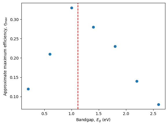
Discusion
Silicon is used in solar cells because its bandgap allows a very efficient photovoltaic conversion of the sunlight as the overall transmission and thermalization losses are minimized, or, in other words, the trade-off between high current and voltage is maximized.