import numpy as np
import matplotlib.pyplot as plt
import math
DATA_SIZE = 1000
kB = 8.617333e-5
q = 1.6021766e-19 #eV
#Material data
D0 = 10.5 #cm2·s-1
Ea = 3.69 #eV
mu = 1500 #cm2/V·s
Nwafer = 1e17 #cm-3
#Process data
T_list = np.array([900, 900, 900], dtype='double') #ºC
time_list = np.array([600, 1200, 1800], dtype='double') #s
Ns = 3e20 #cm-3
depth = 0.05e-4# cm
# Define intermediate profiles to plot
plot_profile = [1, 1, 1]
### Calculate profiles
# Temperatures in K
T_list += 273.15 #K
nSteps = len(T_list)
# Make array with constant base doping profile
Nbase = np.zeros((DATA_SIZE,2))
Nbase[:,0] = np.linspace(0, depth, DATA_SIZE)
Nbase[:,1] = Nwafer
# Make array for profiles calculated
Nx = np.zeros((DATA_SIZE,2))
Nx[:,0] = np.linspace(0, depth, DATA_SIZE)
# Array with depths in microns for plotting
depth_um = np.zeros((DATA_SIZE))
depth_um = Nx[:,0]*1e4
# 1. Predeposition
# First point in list of steps is assumed to be a predeposition
dif_coef = D0*math.exp(-Ea/(kB*T_list[0]))
dif_len = math.sqrt(4*dif_coef*time_list[0])
for x in range(DATA_SIZE):
Nx[x,1] = Ns*math.erfc(Nx[x,0]/dif_len)
linestyles = ('-', '--', '-.', ':')
fig = plt.figure(figsize=[5,4], tight_layout=True)
ax = fig.add_subplot()
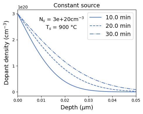
ax.set_title('Constant source', size=14)
fig.text(0.43, 0.85, 'N$_{s}$ = '+ f"{Ns:.3}" + 'cm$^{-3}$',horizontalalignment='center',
verticalalignment='top', fontsize=13)
fig.text(0.43, 0.78, 'T$_{s}$ = '+ f"{T_list[0]-273.15:.0f}" + ' °C',horizontalalignment='center',
verticalalignment='top', fontsize=13)
ax.set_xlabel('Depth ($\mu$m)', size=14)
ax.set_ylabel('Dopant density (cm$^{-3}$)', size=14)
#ax.set_yscale('log')
#ax.set_ylim(Nwafer/10, Ns*10)
ax.set_xlim(0, depth*1e4)
plt.rc('xtick', labelsize=16)
plt.rc('ytick', labelsize=16)
#
#
for x in range(nSteps):
dif_coef = D0*math.exp(-Ea/(kB*T_list[x]))
dif_len = math.sqrt(4*dif_coef*time_list[x])
for y in range(DATA_SIZE):
Nx[y,1] = Ns*math.erfc(Nx[y,0]/dif_len)
Qload = Ns*dif_len/math.sqrt(math.pi)
x_junc = dif_len*(math.erfc(Nwafer/Ns))**-1
Rsheet = 1/(q*mu*Qload)
print("Q = "+f"{Qload:.3}"+" cm3")
print("Rsheet = "+f"{Rsheet:.3f}"+" ohm/sq")
# dif_len = 0
# for z in range(x+1):
# dif_coef = D0*math.exp(-Ea/(kB*T_list[z+1]))
# dif_len += dif_coef*time_list[z+1]
# dif_len = 2*math.sqrt(dif_len)
# for y in range(DATA_SIZE):
# Nx[y,1] = (2/math.sqrt(math.pi))*(Qload/dif_len)*math.exp(-(Nx[y,0]/dif_len)**2)
if plot_profile[x]==1:
trace, = ax.plot(depth_um, Nx[:,1], color='#4472C4', linestyle=linestyles[x], label=str(time_list[x]/60) + ' min')
ax.legend(fontsize=14)
plt.savefig("fig_constantSource.png", dpi=300)