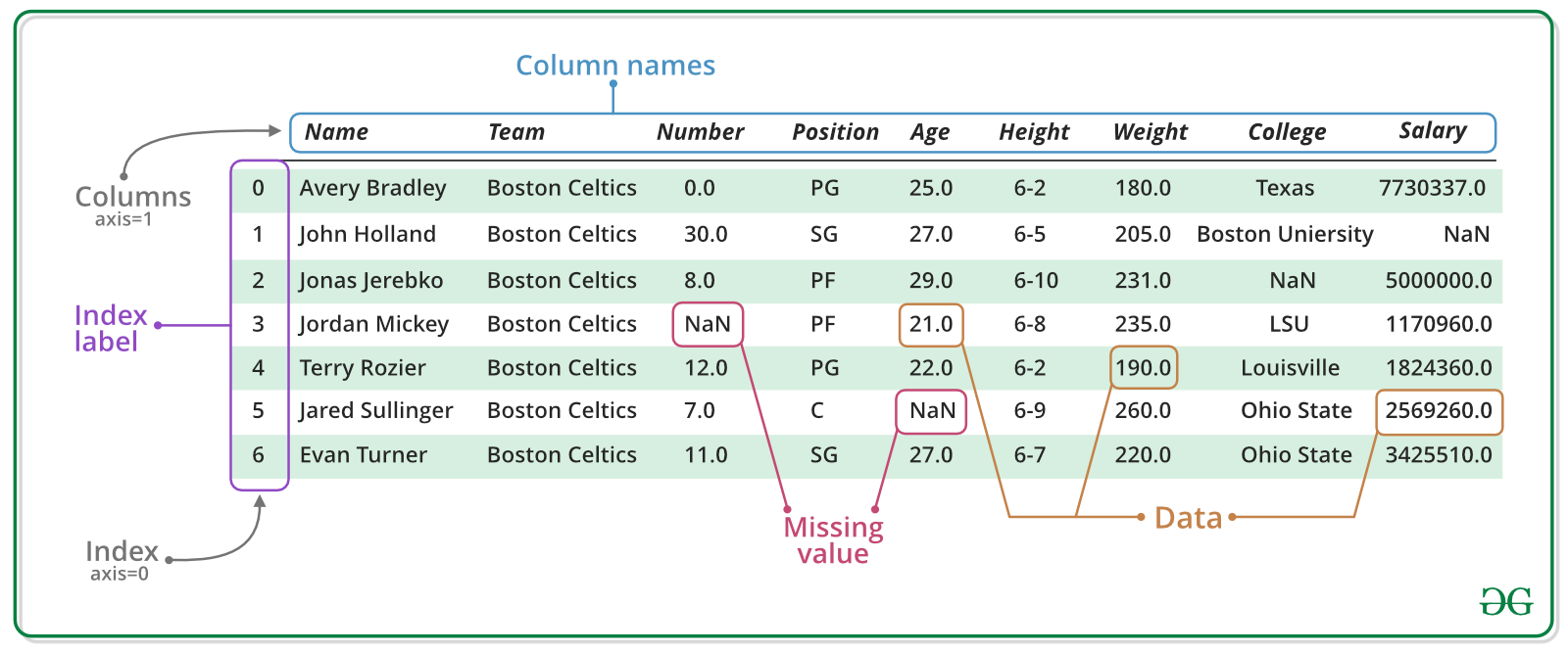
Introduction to pandas

Introduction to `pandas`#

Note

This material is mostly adapted from the following resources:

Pandas is a an open source library providing high-performance, easy-to-use data structures and data analysis tools. Pandas is particularly suited to the analysis of tabular data, i.e. data that can can go into a table. In other words, if you can imagine the data in an Excel spreadsheet, then Pandas is the tool for the job.

A fast and efficient DataFrame object for data manipulation with indexing;
Tools for reading and writing data: CSV and text files, Excel, SQL;
Intelligent data alignment and integrated handling of missing data;
Flexible reshaping and pivoting of data sets;
Intelligent label-based slicing, indexing, and subsetting of large data sets;
High performance aggregating, merging, joining or transforming data;
Hierarchical indexing provides an intuitive way of working with high-dimensional data;
Time series-functionality: date-based indexing, frequency conversion, moving windows, date shifting and lagging;

Note

Documentation for this package is available at https://pandas.pydata.org/docs/.

Note

If you have not yet set up Python on your computer, you can execute this tutorial in your browser via Google Colab. Click on the rocket in the top right corner and launch “Colab”. If that doesn’t work download the .ipynb file and import it in Google Colab.

Then install pandas and numpy by executing the following command in a Jupyter cell at the top of the notebook.

!pip install pandas numpy

import pandas as pd
import numpy as np

Pandas Data Structures: Series#

A Series represents a one-dimensional array of data. The main difference between a Series and numpy array is that a Series has an index. The index contains the labels that we use to access the data.

There are many ways to create a Series. We will just show a few. The core constructor is pd.Series().

(Data are from Wikipedia’s List of photovoltaic power stations.)

names = ["Gonghe Talatan", "Midong","Bhadla"]
values = [10380, 3500, 2245]
s = pd.Series(values, index=names)
s

Gonghe Talatan    10380
Midong             3500
Bhadla             2245
dtype: int64

dictionary = {
    "Gonghe Talatan": 10380, 
    "Midong": 3500,
    "Bhadla": 2245
}
s = pd.Series(dictionary)
s

Gonghe Talatan    10380
Midong             3500
Bhadla             2245
dtype: int64

Arithmetic operations and most numpy functions can be applied to pd.Series. An important point is that the Series keep their index during such operations.

np.log(s) / s**0.5

Gonghe Talatan    0.090768
Midong            0.137938
Bhadla            0.162858
dtype: float64

We can access the underlying index object if we need to:

s.index

Index(['Gonghe Talatan', 'Midong', 'Bhadla'], dtype='object')

We can get values back out using the index via the .loc attribute

s.loc["Bhadla"]

Or by raw position using .iloc

s.iloc[2]

We can pass a list or array to loc to get multiple rows back:

s.loc[['Gonghe Talatan', 'Midong']]

Gonghe Talatan    10380
Midong             3500
dtype: int64

And we can even use slice notation

s.loc['Gonghe Talatan': 'Midong']

Gonghe Talatan    10380
Midong             3500
dtype: int64

s.iloc[:2]

Gonghe Talatan    10380
Midong             3500
dtype: int64

If we need to, we can always get the raw data back out as well

s.values  # a numpy array

array([10380,  3500,  2245])

Pandas Data Structures: DataFrame#

There is a lot more to Series, but they are limit to a single column. A more useful Pandas data structure is the DataFrame. A DataFrame is basically a bunch of series that share the same index. It’s a lot like a table in a spreadsheet.

The core constructor is pd.DataFrame()

Below we create a DataFrame.

# first we create a dictionary
data = {
    "capacity": [10380,  3500,  2245],  # MW
    "type": ["photovoltaic", "photovoltaic", "photovoltaic"],
    "start_year": [2023, 2024, 2018],
    "end_year": [np.nan, np.nan, np.nan],
}
df = pd.DataFrame(data, index=["Gonghe Talatan", "Midong","Bhadla"])
df

	capacity	type	start_year	end_year
Gonghe Talatan	10380	photovoltaic	2023	NaN
Midong	3500	photovoltaic	2024	NaN
Bhadla	2245	photovoltaic	2018	NaN

We can also switch columns and rows very easily.

df.T

	Gonghe Talatan	Midong	Bhadla
capacity	10380	3500	2245
type	photovoltaic	photovoltaic	photovoltaic
start_year	2023	2024	2018
end_year	NaN	NaN	NaN

A wide range of statistical functions are available on both Series and DataFrames.

df.min()

capacity              2245
type          photovoltaic
start_year            2018
end_year               NaN
dtype: object

df.mean(numeric_only=True)

capacity      5375.000000
start_year    2021.666667
end_year              NaN
dtype: float64

df.std(numeric_only=True)

capacity      4379.64325
start_year       3.21455
end_year             NaN
dtype: float64

df.describe()

	capacity	start_year	end_year
count	3.00000	3.000000	0.0
mean	5375.00000	2021.666667	NaN
std	4379.64325	3.214550	NaN
min	2245.00000	2018.000000	NaN
25%	2872.50000	2020.500000	NaN
50%	3500.00000	2023.000000	NaN
75%	6940.00000	2023.500000	NaN
max	10380.00000	2024.000000	NaN

We can get a single column as a Series using python’s getitem syntax on the DataFrame object.

df["capacity"]

Gonghe Talatan    10380
Midong             3500
Bhadla             2245
Name: capacity, dtype: int64

…or using attribute syntax.

df.capacity

Gonghe Talatan    10380
Midong             3500
Bhadla             2245
Name: capacity, dtype: int64

Indexing works very similar to series

df.loc["Bhadla"]

capacity              2245
type          photovoltaic
start_year            2018
end_year               NaN
Name: Bhadla, dtype: object

df.iloc[2]

capacity              2245
type          photovoltaic
start_year            2018
end_year               NaN
Name: Bhadla, dtype: object

But we can also specify the column(s) and row(s) we want to access

df.loc["Bhadla", "start_year"]

df.loc[["Midong", "Bhadla"], ["start_year", "end_year"]]

	start_year	end_year
Midong	2024	NaN
Bhadla	2018	NaN

df.capacity * 0.8

Gonghe Talatan    8304.0
Midong            2800.0
Bhadla            1796.0
Name: capacity, dtype: float64

Which we can easily add as another column to the DataFrame:

df["reduced_capacity"] = df.capacity * 0.8
df

	capacity	type	start_year	end_year	reduced_capacity
Gonghe Talatan	10380	photovoltaic	2023	NaN	8304.0
Midong	3500	photovoltaic	2024	NaN	2800.0
Bhadla	2245	photovoltaic	2018	NaN	1796.0

We can also remove columns or rows from a DataFrame:

df.drop("reduced_capacity", axis="columns")

	capacity	type	start_year	end_year
Gonghe Talatan	10380	photovoltaic	2023	NaN
Midong	3500	photovoltaic	2024	NaN
Bhadla	2245	photovoltaic	2018	NaN

We can update the variable df by either overwriting df or passing an inplace keyword:

df.drop("reduced_capacity", axis="columns", inplace=True)

We can also drop columns with only NaN values

df.dropna(axis=1)

	capacity	type	start_year
Gonghe Talatan	10380	photovoltaic	2023
Midong	3500	photovoltaic	2024
Bhadla	2245	photovoltaic	2018

Or fill it up with default “fallback” data:

df.fillna(2050)

	capacity	type	start_year	end_year
Gonghe Talatan	10380	photovoltaic	2023	2050.0
Midong	3500	photovoltaic	2024	2050.0
Bhadla	2245	photovoltaic	2018	2050.0

Say, we already have one value for end_year and want to fill up the missing data:

df.loc["Bhadla", "end_year"] = 2050

# backward (upwards) fill from non-nan values
df.fillna(method="bfill")

/tmp/ipykernel_3504/532230991.py:2: FutureWarning: DataFrame.fillna with 'method' is deprecated and will raise in a future version. Use obj.ffill() or obj.bfill() instead.
  df.fillna(method="bfill")

	capacity	type	start_year	end_year
Gonghe Talatan	10380	photovoltaic	2023	2050.0
Midong	3500	photovoltaic	2024	2050.0
Bhadla	2245	photovoltaic	2018	2050.0

Sorting Data#

We can also sort the entries in dataframes, e.g. alphabetically by index or numerically by column values

df.sort_index()

	capacity	type	start_year	end_year
Bhadla	2245	photovoltaic	2018	2050.0
Gonghe Talatan	10380	photovoltaic	2023	NaN
Midong	3500	photovoltaic	2024	NaN

df.sort_values(by="capacity", ascending=False)

	capacity	type	start_year	end_year
Gonghe Talatan	10380	photovoltaic	2023	NaN
Midong	3500	photovoltaic	2024	NaN
Bhadla	2245	photovoltaic	2018	2050.0

If we make a calculation using columns from the DataFrame, it will keep the same index:

Merging Data#

Pandas supports a wide range of methods for merging different datasets. These are described extensively in the documentation. Here we just give a few examples.

data = {
    "capacity": [2050, 1650, 1350],  # MW
    "type": ["photovoltaic", "photovoltaic","photovoltaic",],
    "start_year": [2019, 2019, 2021],
}
df2 = pd.DataFrame(data, index=["Pavagada", "Benban", "Kalyon Karapinar"])
df2

	capacity	type	start_year
Pavagada	2050	photovoltaic	2019
Benban	1650	photovoltaic	2019
Kalyon Karapinar	1350	photovoltaic	2021

We can now add this additional data to the df object

df = pd.concat([df, df2])
df

	capacity	type	start_year	end_year
Gonghe Talatan	10380	photovoltaic	2023	NaN
Midong	3500	photovoltaic	2024	NaN
Bhadla	2245	photovoltaic	2018	2050.0
Pavagada	2050	photovoltaic	2019	NaN
Benban	1650	photovoltaic	2019	NaN
Kalyon Karapinar	1350	photovoltaic	2021	NaN

Filtering Data#

We can also filter a DataFrame using a boolean series obtained from a condition. This is very useful to build subsets of the DataFrame.

df.capacity > 2000

Gonghe Talatan       True
Midong               True
Bhadla               True
Pavagada             True
Benban              False
Kalyon Karapinar    False
Name: capacity, dtype: bool

df[df.capacity > 2000]

	capacity	type	start_year	end_year
Gonghe Talatan	10380	photovoltaic	2023	NaN
Midong	3500	photovoltaic	2024	NaN
Bhadla	2245	photovoltaic	2018	2050.0
Pavagada	2050	photovoltaic	2019	NaN

We can also combine multiple conditions, but we need to wrap the conditions with brackets!

df[(df.capacity > 2000) & (df.start_year >= 2020)]

	capacity	type	start_year	end_year
Gonghe Talatan	10380	photovoltaic	2023	NaN
Midong	3500	photovoltaic	2024	NaN

Or we make SQL-like queries:

df.query("start_year == 2019")

	capacity	type	start_year	end_year
Pavagada	2050	photovoltaic	2019	NaN
Benban	1650	photovoltaic	2019	NaN

threshold = 2000
df.query("start_year == 2019 and capacity > @threshold")

	capacity	type	start_year	end_year
Pavagada	2050	photovoltaic	2019	NaN

Modifying Values#

In many cases, we want to modify values in a dataframe based on some rule. To modify values, we need to use .loc or .iloc

df.loc["Bhadla", "capacity"] += 500
df

	capacity	type	start_year	end_year
Gonghe Talatan	10380	photovoltaic	2023	NaN
Midong	3500	photovoltaic	2024	NaN
Bhadla	2745	photovoltaic	2018	2050.0
Pavagada	2050	photovoltaic	2019	NaN
Benban	1650	photovoltaic	2019	NaN
Kalyon Karapinar	1350	photovoltaic	2021	NaN

Applying Functions#

Sometimes it can be useful apply a function to all values of a column/row. For instance, we might be interested in normalised capacities relative to the largest PV power plant:

df.capacity.apply(lambda x: x / df.capacity.max())

Gonghe Talatan      1.000000
Midong              0.337187
Bhadla              0.264451
Pavagada            0.197495
Benban              0.158960
Kalyon Karapinar    0.130058
Name: capacity, dtype: float64

df.capacity.map(lambda x: x / df.capacity.max())

Gonghe Talatan      1.000000
Midong              0.337187
Bhadla              0.264451
Pavagada            0.197495
Benban              0.158960
Kalyon Karapinar    0.130058
Name: capacity, dtype: float64

For simple functions, there’s often an easier alternative:

df.capacity / df.capacity.max()

Gonghe Talatan      1.000000
Midong              0.337187
Bhadla              0.264451
Pavagada            0.197495
Benban              0.158960
Kalyon Karapinar    0.130058
Name: capacity, dtype: float64

But .apply() and .map() often give you more flexibility.

Renaming Indices and Columns#

Sometimes it can be useful to rename columns:

df.rename(columns=dict(start_year="commission", end_year="decommission"))

	capacity	type	commission	decommission
Gonghe Talatan	10380	photovoltaic	2023	NaN
Midong	3500	photovoltaic	2024	NaN
Bhadla	2745	photovoltaic	2018	2050.0
Pavagada	2050	photovoltaic	2019	NaN
Benban	1650	photovoltaic	2019	NaN
Kalyon Karapinar	1350	photovoltaic	2021	NaN

Replacing Values#

Sometimes it can be useful to replace values:

df.replace({"photovoltaic": "PV"})

	capacity	type	start_year	end_year
Gonghe Talatan	10380	PV	2023	NaN
Midong	3500	PV	2024	NaN
Bhadla	2745	PV	2018	2050.0
Pavagada	2050	PV	2019	NaN
Benban	1650	PV	2019	NaN
Kalyon Karapinar	1350	PV	2021	NaN

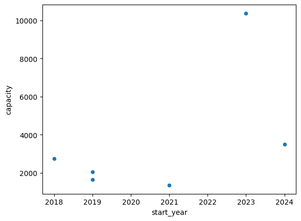
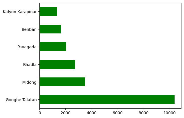
Plotting#

DataFrames have all kinds of useful plotting built in. Note that we do not even have to import matplotlib for this.

df.plot(kind="scatter", x="start_year", y="capacity")

<Axes: xlabel='start_year', ylabel='capacity'>

_images/caef6c016a2c59346960fe197de4e265e44dd703352b06984cfa89cea6d844a7.png

df.capacity.plot.barh(color="green")

<Axes: >

_images/888dd98aa96c0e514a7bd707618f23dc419fe3402e5263b3b57c716ad09ac060.png

Reading and Writing Files#

To read data into pandas, we can use for instance the pd.read_csv() function. This function is incredibly powerful and complex with a multitude of settings. You can use it to extract data from almost any text file.

The pd.read_csv() function can take a path to a local file as an input, or even a link to an online text file.

Let’s import a file containing data measured at a weather station.

fn = "weather_station_data.csv"

df = pd.read_csv(fn, index_col=0)
df.iloc[:5, :10]

	GHI (W.m-2)	DHI (W.m-2)	Ambient Temperature (Deg C)	Relative Humidity (%)	wind velocity (m.s-1)	wind direction (deg)
2024-01-01 00:00:00+00:00	3.290	2.187	5.428	95.4	2.409	120.8
2024-01-01 00:05:00+00:00	3.201	2.013	5.425	95.4	2.951	123.8
2024-01-01 00:10:00+00:00	3.308	2.203	5.456	95.5	2.648	124.9
2024-01-01 00:15:00+00:00	3.010	1.796	5.470	95.5	2.723	122.0
2024-01-01 00:20:00+00:00	3.479	2.370	5.491	95.4	2.478	125.5

df.info()

<class 'pandas.core.frame.DataFrame'>
Index: 52704 entries, 2024-01-01 00:00:00+00:00 to 2024-07-01 23:55:00+00:00
Data columns (total 6 columns):
 #   Column                       Non-Null Count  Dtype  
---  ------                       --------------  -----  
 0   GHI (W.m-2)                  52249 non-null  float64
 1   DHI (W.m-2)                  52249 non-null  float64
 2   Ambient Temperature (Deg C)  52249 non-null  float64
 3   Relative Humidity (%)        52249 non-null  float64
 4   wind velocity (m.s-1)        52274 non-null  float64
 5   wind direction (deg)         52274 non-null  float64
dtypes: float64(6)
memory usage: 2.8+ MB

df.describe()

	GHI (W.m-2)	DHI (W.m-2)	Ambient Temperature (Deg C)	Relative Humidity (%)	wind velocity (m.s-1)	wind direction (deg)
count	52249.000000	52249.000000	52249.000000	52249.000000	52274.000000	52274.000000
mean	125.476227	64.949393	7.658637	81.494715	2.822048	172.038209
std	205.015278	94.282571	6.425798	13.194039	1.618026	91.322030
min	0.933000	0.474000	-13.290000	27.650000	0.000000	0.000000
25%	3.631000	2.414000	3.609000	75.200000	1.630250	93.600000
50%	13.220000	11.850000	7.053000	85.400000	2.629000	174.900000
75%	158.400000	94.900000	11.930000	91.200000	3.779000	248.600000
max	1246.000000	645.100000	26.710000	100.000000	13.180000	360.000000

Sometimes, we also want to store a DataFrame for later use. There are many different file formats tabular data can be stored in, including HTML, JSON, Excel, Parquet, Feather, etc. Here, let’s say we want to store the DataFrame as CSV (comma-separated values) file under the name “data.csv”.

df.to_csv("data.csv")

Introduction to pandas

Contents

Introduction to pandas#

Pandas Data Structures: Series#

Pandas Data Structures: DataFrame#

Sorting Data#

Merging Data#

Filtering Data#

Modifying Values#

Applying Functions#

Renaming Indices and Columns#

Replacing Values#

Plotting#

Reading and Writing Files#

Introduction to `pandas`#