Problem 3.4

Fundamentals of Solar Cells and Photovoltaic Systems Engineering

Solutions Manual - Chapter 3

Problem 3.4

The refractive index of silicon at 25°C can be found in the file “Refractive index silicon.csv” in the online repository of the book.

(a) Calculate and plot the reflectance \(r\) at the front surface of a silicon solar cell as a function of the photon wavelength.

(b) Plot the QE of an ideal silicon solar cell and the QE of a silicon solar cell assuming that it is ideal except for the reflection losses. Discuss the results.

We will use the package pandas to handle the data and matplotlib.pyplot to plot the results

import pandas as pd
import numpy as np
import matplotlib.pyplot as plt

We start by importing the data.

datafile = pd.read_csv('data/Refractive index silicon.csv', index_col=0, header=0) 
datafile

	n_Si_25C
nm	NaN
250	1.6640
260	1.7540
270	2.0870
280	2.9610
...	...
1410	3.4928
1420	3.4917
1430	3.4906
1440	3.4896
1450	3.4885

122 rows × 1 columns

datafile.drop(datafile.index[0], inplace=True) #remove row including information on units
datafile=datafile.astype(float) #convert values to float for easy operation
datafile.index=datafile.index.astype(float) #convert indexees to float for easy operation

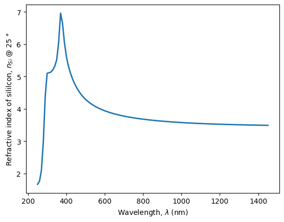
We visualize the refectrative index spectra.

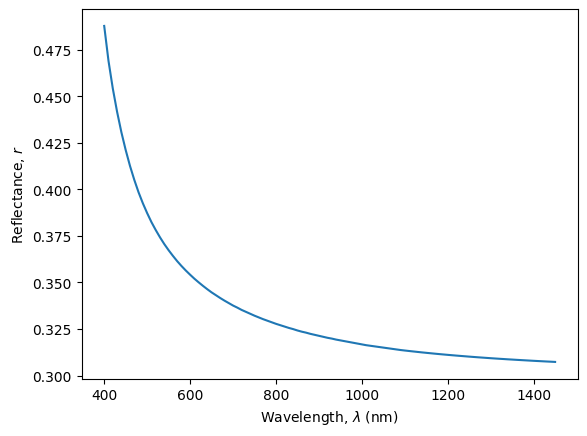
We calculate the reflectance at the air/silicon interface using Eq. 3.9 and plot it.

\(r=[\frac{(n_{Si}-1)}{(n_{Si}+1)}]^2\)

plt.plot(datafile, 
         linewidth=2)
plt.ylabel(r'Refractive index of sililcon, $n_{Si}$ @ 25 $\degree$')
plt.xlabel('Wavelength, $\lambda$ (nm)')

Text(0.5, 0, 'Wavelength, $\\lambda$ (nm)')

n=datafile['n_Si_25C'][datafile.index>=400]
r=((n-1)/(n+1))**2
plt.plot(r)
plt.ylabel(r'Reflectance, $r$')
plt.xlabel('Wavelength, $\lambda$ (nm)')

Text(0.5, 0, 'Wavelength, $\\lambda$ (nm)')

(b) Plot the QE of an ideal silicon solar cell and the QE of a silicon solar cell assuming that it is ideal except for the reflection losses. Discuss the results.

The ideal QE is 1 for wavelengths shorter than the bandgap wavelength \(\lambda_g\) and 0 for longer wavelengths.

bg_wl=1240/1.12
QEone=lambda x: 1 if x < bg_wl else 0
ideal_QE=pd.Series(index=r.index,
                   data=[QEone(i) for i in r.index])

To account for the reflection losses, the ideal QE is multiplied by (1-\(r\))

QE_ref_loss=pd.Series(index=ideal_QE.index,
                    data=[(1-r.loc[i])*ideal_QE.loc[i] for i in ideal_QE.index])

We plot the ideal QE and the actual QE (affected by \(r\))

plt.plot(ideal_QE,
         linewidth=2, label='ideal')
plt.plot(QE_ref_loss,
         linewidth=2, label='with reflection')
plt.ylabel(r'Quantum Efficiency, $QE$')
plt.xlabel('Wavelength, $\lambda$ (nm)')
plt.legend()

<matplotlib.legend.Legend at 0x7f725144f550>

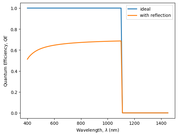
Discussion

The reflecion losses reduce the QE and hence the photocurrent.
In silicon, these losses are higher than 30% for all wavelenghts, and are specially higher at short wavelenghts (<600 nm) becasue of the fast increase of the refractive index of silicon in that wavelength range.