Problem 11.2

Integrated Energy Grids

Problem 11.2. Join capacity and dispatch optimization.

Create a model in PyPSA and optimize the capacity and dispatch of solar PV, onshore wind and battery storage to supply the inelastic electricity demand throughout the year, including demand assuming full electrification of land transport. To do this, take the time series for the wind and solar capacity factors for Portugal in 2015 and the electricity demand.

Assume that the 5.6 million cars currently existing in Portugal are replaced by electric vehicles (EVs), with an average EV battery capacity of 50 kWh and a charging capacity of 11 kV. The time series for EV electricity demand can be found in the course repository.

a) If EV batteries are assumed to be charged right after the cars are used, calculate the required capacity and generation mix for the optimal system. Plot the energy generation and demand throughout July 1st. The EVs can only be charged when they are parked, and this can be represented by the availability profile.

Note

If you have not yet set up Python on your computer, you can execute this tutorial in your browser via Google Colab. Click on the rocket in the top right corner and launch “Colab”. If that doesn’t work download the .ipynb file and import it in Google Colab.

Then install pandas and numpy by executing the following command in a Jupyter cell at the top of the notebook.

!pip install pandas pypsa

import matplotlib.pyplot as plt
import pandas as pd
import pypsa

Prerequisites: handling technology data and costs

We maintain a database (PyPSA/technology-data) which collects assumptions and projections for energy system technologies (such as costs, efficiencies, lifetimes, etc.) for given years, which we can load into a pandas.DataFrame. This requires some pre-processing to load (e.g. converting units, setting defaults, re-arranging dimensions):

year = 2030
url = f"https://raw.githubusercontent.com/PyPSA/technology-data/master/outputs/costs_{year}.csv"
costs = pd.read_csv(url, index_col=[0, 1])

costs.loc[costs.unit.str.contains("/kW"), "value"] *= 1e3
costs.unit = costs.unit.str.replace("/kW", "/MW")

defaults = {
    "FOM": 0,
    "VOM": 0,
    "efficiency": 1,
    "fuel": 0,
    "investment": 0,
    "lifetime": 25,
    "CO2 intensity": 0,
    "discount rate": 0.07,
}
costs = costs.value.unstack().fillna(defaults)

costs.at["OCGT", "fuel"] = costs.at["gas", "fuel"]
costs.at["OCGT", "CO2 intensity"] = costs.at["gas", "CO2 intensity"]

Let’s also write a small utility function that calculates the annuity to annualise investment costs. The formula is

\[ a(r, n) = \frac{r}{1-(1+r)^{-n}} \]

where \(r\) is the discount rate and \(n\) is the lifetime.

def annuity(r, n):
    return r / (1.0 - 1.0 / (1.0 + r) ** n)

annuity(0.07, 20)

0.09439292574325567

Based on this, we can calculate the marginal generation costs (€/MWh):

costs["marginal_cost"] = costs["VOM"] + costs["fuel"] / costs["efficiency"]

and the annualised investment costs (capital_cost in PyPSA terms, €/MW/a):

annuity = costs.apply(lambda x: annuity(x["discount rate"], x["lifetime"]), axis=1)

costs["capital_cost"] = (annuity + costs["FOM"] / 100) * costs["investment"]

We can now read the capital and marginal cost of onshore wind and solar.

costs.at["onwind", "capital_cost"] #EUR/MW/a

np.float64(101644.12332388277)

costs.at["solar", "capital_cost"] #EUR/MW/a

np.float64(51346.82981964593)

Retrieving time series data

In this example, wind data from https://zenodo.org/record/3253876#.XSiVOEdS8l0 and solar PV data from https://zenodo.org/record/2613651#.X0kbhDVS-uV is used. The data is downloaded in csv format and saved in the ‘data’ folder. The Pandas package is used as a convenient way of managing the datasets.

For convenience, the column including date information is converted into Datetime and set as index

data_solar = pd.read_csv('data/pv_optimal.csv',sep=';')
data_solar.index = pd.DatetimeIndex(data_solar['utc_time'])

data_wind = pd.read_csv('data/onshore_wind_1979-2017.csv',sep=';')
data_wind.index = pd.DatetimeIndex(data_wind['utc_time'])

data_el = pd.read_csv('data/electricity_demand.csv',sep=';')
data_el.index = pd.DatetimeIndex(data_el['utc_time'])

data_el_EV = pd.read_csv('data/EV_electricity_demand.csv',sep=';')
data_el_EV.index = pd.DatetimeIndex(data_el_EV['utc_time'])

The data format can now be analyzed using the .head() function to show the first lines of the data set

data_el_EV.head()

	utc_time	PRT
utc_time
2015-01-01 00:00:00+00:00	2015-01-01T00:00:00Z	703.395764
2015-01-01 01:00:00+00:00	2015-01-01T01:00:00Z	474.707583
2015-01-01 02:00:00+00:00	2015-01-01T02:00:00Z	359.721755
2015-01-01 03:00:00+00:00	2015-01-01T03:00:00Z	344.947896
2015-01-01 04:00:00+00:00	2015-01-01T04:00:00Z	436.246018

We will use timeseries for Portugal in this excercise

country = 'PRT'

Join capacity and dispatch optimization

For building the model, we start again by initialising an empty network, adding the snapshots, the electricity and the EV bus.

n = pypsa.Network()
hours_in_2015 = pd.date_range('2015-01-01 00:00Z',
                              '2015-12-31 23:00Z',
                              freq='h')

n.set_snapshots(hours_in_2015.values)

n.add("Bus", "electricity")
n.add("Bus", "EV")

Index(['EV'], dtype='object')

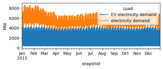
Next, we add the demand time series to the model.

# add load to the bus
n.add("Load",
      "electricity demand",
      bus="electricity",
      p_set=data_el[country].values)

Index(['electricity demand'], dtype='object')

We can add now the electricity demand from EVs and check that it was properly added.

# add load to the bus
n.add("Load",
      "EV electricity demand",
      bus="EV",
      p_set=data_el_EV[country].values)

n.loads_t.p_set.plot(figsize=(6, 2), ylabel="MW")

<Axes: xlabel='snapshot', ylabel='MW'>

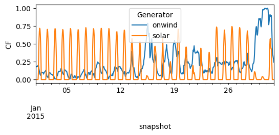
We add now the generators and set up their capacities to be extendable so that they can be optimized together with the dispatch time series. For the wind and solar generator, we need to indicate the capacity factor or maximum power per unit ‘p_max_pu’

CF_wind = data_wind[country][[hour.strftime("%Y-%m-%dT%H:%M:%SZ") for hour in n.snapshots]]
n.add(
        "Generator",
        "onwind",
        bus="electricity",
        carrier="onwind",
        p_max_pu=CF_wind.values,
        capital_cost=costs.at["onwind", "capital_cost"],
        marginal_cost=costs.at["onwind", "marginal_cost"],
        efficiency=costs.at["onwind", "efficiency"],
        p_nom_extendable=True,
    )

CF_solar = data_solar[country][[hour.strftime("%Y-%m-%dT%H:%M:%SZ") for hour in n.snapshots]]
n.add(
        "Generator",
        "solar",
        bus="electricity",
        carrier="solar",
        p_max_pu= CF_solar.values,
        capital_cost=costs.at["solar", "capital_cost"],
        marginal_cost=costs.at["solar", "marginal_cost"],
        efficiency=costs.at["solar", "efficiency"],
        p_nom_extendable=True,
    )

Index(['solar'], dtype='object')

So let’s make sure the capacity factors are read-in correctly.

n.generators_t.p_max_pu.loc["2015-01"].plot(figsize=(6, 2), ylabel="CF")

<Axes: xlabel='snapshot', ylabel='CF'>

We add the battery storage, assuming a fixed energy-to-power ratio of 6 hours, i.e. if fully charged, the battery can discharge at full capacity for 6 hours.

For capital costs, we have to factor in both the capacity and energy costs of storage.

We include the charging and discharging efficiencies we enforce a cyclic state-of-charge condition, i.e. the state of charge at the beginning of the optimisation period must equal the final state of charge.

n.add(
    "StorageUnit",
    "battery storage",
    bus="electricity",
    carrier="battery storage",
    max_hours=6,
    capital_cost=costs.at["battery inverter", "capital_cost"]
    + 6 * costs.at["battery storage", "capital_cost"],
    efficiency_store=costs.at["battery inverter", "efficiency"],
    efficiency_dispatch=costs.at["battery inverter", "efficiency"],
    p_nom_extendable=True,
    cyclic_state_of_charge=True,
)

Index(['battery storage'], dtype='object')

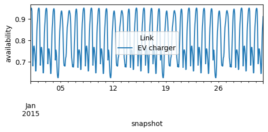
The electric vehicles can only be charged when they are plugged-in. Below we load an availability profile telling us what share of electric vehicles is plugged-in at home – we only assume home charging in this example.

Then, we can add a link for the electric vehicle charger using an assumption about the number of EVs and their charging capacity

EV_availability_profile = pd.read_csv('data/EV_availability.csv',sep=';')
EV_availability_profile.index = pd.DatetimeIndex(EV_availability_profile['utc_time'])

number_cars = 5600000 #  number of EV cars
bev_charger_rate = 0.011  # 11 kW -> MW
p_nom = number_cars * bev_charger_rate

n.add(
    "Link",
    "EV charger",
    bus0="electricity",
    bus1="EV",
    p_nom=p_nom,
    p_max_pu=EV_availability_profile['PRT'].values,
    efficiency=0.9,
)

n.links_t.p_max_pu.loc["2015-01"].plot(figsize=(6, 2), ylabel="availability")

<Axes: xlabel='snapshot', ylabel='availability'>

Model Run

We can already solve the model using the open-solver “highs” or the commercial solver “gurobi” with the academic license

n.optimize(solver_name="highs")

WARNING:pypsa.consistency:The following generators have carriers which are not defined:
Index(['onwind', 'solar'], dtype='object', name='Generator')

WARNING:pypsa.consistency:The following buses have carriers which are not defined:
Index(['electricity', 'EV'], dtype='object', name='Bus')

WARNING:pypsa.consistency:The following storage_units have carriers which are not defined:
Index(['battery storage'], dtype='object', name='StorageUnit')

WARNING:pypsa.consistency:The following links have carriers which are not defined:
Index(['EV charger'], dtype='object', name='Link')

INFO:linopy.model: Solve problem using Highs solver

INFO:linopy.io:Writing objective.

Writing constraints.:   0%|          | 0/16 [00:00<?, ?it/s]

Writing constraints.:  38%|███▊      | 6/16 [00:00<00:00, 47.13it/s]

Writing constraints.:  69%|██████▉   | 11/16 [00:00<00:00, 40.64it/s]

Writing constraints.: 100%|██████████| 16/16 [00:00<00:00, 26.61it/s]

Writing constraints.: 100%|██████████| 16/16 [00:00<00:00, 29.81it/s]

Writing continuous variables.:   0%|          | 0/7 [00:00<?, ?it/s]

Writing continuous variables.: 100%|██████████| 7/7 [00:00<00:00, 75.30it/s]

INFO:linopy.io: Writing time: 0.66s

Running HiGHS 1.10.0 (git hash: fd86653): Copyright (c) 2025 HiGHS under MIT licence terms
LP   linopy-problem-pzex_viv has 131403 rows; 52563 cols; 232161 nonzeros
Coefficient ranges:
  Matrix [1e-03, 6e+00]
  Cost   [1e-02, 1e+05]
  Bound  [0e+00, 0e+00]
  RHS    [3e+02, 6e+04]
Presolving model
56958 rows, 39441 cols, 144594 nonzeros  0s
Dependent equations search running on 17520 equations with time limit of 1000.00s
Dependent equations search removed 0 rows and 0 nonzeros in 0.00s (limit = 1000.00s)
56958 rows, 39441 cols, 144594 nonzeros  0s
Presolve : Reductions: rows 56958(-74445); columns 39441(-13122); elements 144594(-87567)
Solving the presolved LP
Using EKK dual simplex solver - serial
  Iteration        Objective     Infeasibilities num(sum)
          0     0.0000000000e+00 Pr: 8760(2.03375e+09) 0s

      33164     8.0098604804e+09 Pr: 0(0); Du: 0(1.38778e-16) 2s
Solving the original LP from the solution after postsolve
Model name          : linopy-problem-pzex_viv
Model status        : Optimal
Simplex   iterations: 33164
Objective value     :  8.0098604804e+09
Relative P-D gap    :  8.8106277989e-15
HiGHS run time      :          1.67
Writing the solution to /tmp/linopy-solve-q359tiol.sol

INFO:linopy.constants: Optimization successful: 
Status: ok
Termination condition: optimal
Solution: 52563 primals, 131403 duals
Objective: 8.01e+09
Solver model: available
Solver message: Optimal

INFO:pypsa.optimization.optimize:The shadow-prices of the constraints Generator-ext-p-lower, Generator-ext-p-upper, Link-fix-p-lower, Link-fix-p-upper, StorageUnit-ext-p_dispatch-lower, StorageUnit-ext-p_dispatch-upper, StorageUnit-ext-p_store-lower, StorageUnit-ext-p_store-upper, StorageUnit-ext-state_of_charge-lower, StorageUnit-ext-state_of_charge-upper, StorageUnit-energy_balance were not assigned to the network.

('ok', 'optimal')

Now, we can look at the results and evaluate the total system cost (in billion Euros per year) and per MWh

n.objective / 1e9

8.009860480443573

n.objective/n.loads_t.p_set.sum().sum()

np.float64(117.1422122888279)

The optimised capacities in GW

n.generators.p_nom_opt.div(1e3)  # MW -> GW

Generator
onwind    25.390863
solar     48.429478
Name: p_nom_opt, dtype: float64

And the optimised static battery capacity

n.storage_units.max_hours*n.storage_units.p_nom_opt.div(1e3) #MWh - GWh

StorageUnit
battery storage    171.403065
dtype: float64

The total energy generation by technology in TWh:

n.generators_t.p.sum().div(1e6)  # MWh -> TWh

Generator
onwind     8.562862
solar     64.449021
dtype: float64

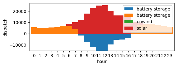
We can plot the dispatch of electricity from every generator throughout January 1st.

date="2015-07-01"
charge = n.storage_units_t.p['battery storage'][n.storage_units_t.p['battery storage']>0].loc[date]
discharge = n.storage_units_t.p['battery storage'][n.storage_units_t.p['battery storage']<0].loc[date]
combined =  pd.concat([discharge, charge, n.generators_t.p.loc[date]], axis=1)

ax = combined.plot.bar(figsize=(6, 2), ylabel="dispatch", xlabel="hour", stacked=True, width=1)
ax.legend(loc='upper right')
ax.set_xticks(range(len(combined.index)))  
ax.set_xticklabels(combined.index.hour, rotation=0) 

[Text(0, 0, '0'),
 Text(1, 0, '1'),
 Text(2, 0, '2'),
 Text(3, 0, '3'),
 Text(4, 0, '4'),
 Text(5, 0, '5'),
 Text(6, 0, '6'),
 Text(7, 0, '7'),
 Text(8, 0, '8'),
 Text(9, 0, '9'),
 Text(10, 0, '10'),
 Text(11, 0, '11'),
 Text(12, 0, '12'),
 Text(13, 0, '13'),
 Text(14, 0, '14'),
 Text(15, 0, '15'),
 Text(16, 0, '16'),
 Text(17, 0, '17'),
 Text(18, 0, '18'),
 Text(19, 0, '19'),
 Text(20, 0, '20'),
 Text(21, 0, '21'),
 Text(22, 0, '22'),
 Text(23, 0, '23')]

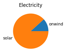
We can also plot the annual electricity mix

n.generators_t.p.sum().plot.pie(figsize=(6, 2), title='Electricity')

<Axes: title={'center': 'Electricity'}>

b) Assume that the EV batteries can be charge when it is optimal for the system (smart-charging). How do the required capacities change relative to section (a)? Plot the energy generation and demand throughout July 1st.

To represent the fact that the EV battery can be charged at any time that is convenient for the system (smart-charging), we add a battery to the EV bus. The energy capacity of that battery is based on the number of vehicles and the assumption of 50 kWh per vehicle.

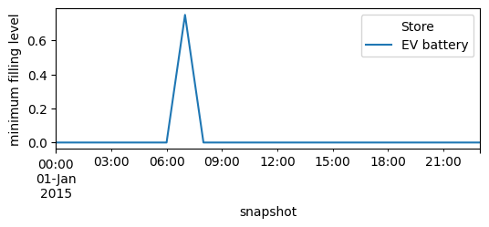
To make sure that this storage behaves as an EV battery, we can impose the requirement that it needs to be charged every morning. (e.g. 75% full every morning).

minimum_filling_level = pd.read_csv('data/EV_minimum_filling_level.csv',sep=';')
minimum_filling_level.index = pd.DatetimeIndex(minimum_filling_level['utc_time'])

bev_energy = 0.05  # average battery size of 1 EV battery in MWh
bev_dsm_participants = 1  # share of cars that do smart charging

e_nom = number_cars * bev_energy * bev_dsm_participants

n.add(
    "Store",
    "EV battery",
    bus="EV",
    e_cyclic=True,  # state of charge at beginning = state of charge at the end
    e_nom=e_nom,
    e_min_pu=minimum_filling_level['PRT'].values,
)

n.stores_t.e_min_pu.loc["2015-01-01"].plot(figsize=(6, 2), ylabel="minimum filling level")

<Axes: xlabel='snapshot', ylabel='minimum filling level'>

n.optimize(solver_name="highs")

WARNING:pypsa.consistency:The following generators have carriers which are not defined:
Index(['onwind', 'solar'], dtype='object', name='Generator')

WARNING:pypsa.consistency:The following stores have carriers which are not defined:
Index(['EV battery'], dtype='object', name='Store')

WARNING:pypsa.consistency:The following buses have carriers which are not defined:
Index(['electricity', 'EV'], dtype='object', name='Bus')

WARNING:pypsa.consistency:The following storage_units have carriers which are not defined:
Index(['battery storage'], dtype='object', name='StorageUnit')

WARNING:pypsa.consistency:The following links have carriers which are not defined:
Index(['EV charger'], dtype='object', name='Link')

INFO:linopy.model: Solve problem using Highs solver

INFO:linopy.io:Writing objective.

Writing constraints.:   0%|          | 0/19 [00:00<?, ?it/s]

Writing constraints.:  32%|███▏      | 6/19 [00:00<00:00, 46.95it/s]

Writing constraints.:  58%|█████▊    | 11/19 [00:00<00:00, 42.82it/s]

Writing constraints.:  84%|████████▍ | 16/19 [00:00<00:00, 35.89it/s]

Writing constraints.: 100%|██████████| 19/19 [00:00<00:00, 28.88it/s]

Writing continuous variables.:   0%|          | 0/9 [00:00<?, ?it/s]

Writing continuous variables.:  89%|████████▉ | 8/9 [00:00<00:00, 74.44it/s]

Writing continuous variables.: 100%|██████████| 9/9 [00:00<00:00, 72.79it/s]

INFO:linopy.io: Writing time: 0.81s

Running HiGHS 1.10.0 (git hash: fd86653): Copyright (c) 2025 HiGHS under MIT licence terms
LP   linopy-problem-18myw0hx has 157683 rows; 70083 cols; 284721 nonzeros
Coefficient ranges:
  Matrix [1e-03, 6e+00]
  Cost   [1e-02, 1e+05]
  Bound  [0e+00, 0e+00]
  RHS    [3e+02, 3e+05]
Presolving model
65718 rows, 56961 cols, 179634 nonzeros  0s
Dependent equations search running on 26280 equations with time limit of 1000.00s
Dependent equations search removed 0 rows and 0 nonzeros in 0.00s (limit = 1000.00s)
65718 rows, 56961 cols, 179634 nonzeros  0s

Presolve : Reductions: rows 65718(-91965); columns 56961(-13122); elements 179634(-105087)
Solving the presolved LP
Using EKK dual simplex solver - serial
  Iteration        Objective     Infeasibilities num(sum)
          0     3.4736136555e+02 Pr: 17520(8.47771e+08) 0s

      60678     6.5754013742e+09 Pr: 0(0); Du: 0(5.56466e-11) 4s
      60678     6.5754013742e+09 Pr: 0(0); Du: 0(5.56466e-11) 4s
Solving the original LP from the solution after postsolve
Model name          : linopy-problem-18myw0hx
Model status        : Optimal
Simplex   iterations: 60678
Objective value     :  6.5754013742e+09
Relative P-D gap    :  1.5954033653e-15
HiGHS run time      :          3.77

INFO:linopy.constants: Optimization successful: 
Status: ok
Termination condition: optimal
Solution: 70083 primals, 157683 duals
Objective: 6.58e+09
Solver model: available
Solver message: Optimal

INFO:pypsa.optimization.optimize:The shadow-prices of the constraints Generator-ext-p-lower, Generator-ext-p-upper, Link-fix-p-lower, Link-fix-p-upper, Store-fix-e-lower, Store-fix-e-upper, StorageUnit-ext-p_dispatch-lower, StorageUnit-ext-p_dispatch-upper, StorageUnit-ext-p_store-lower, StorageUnit-ext-p_store-upper, StorageUnit-ext-state_of_charge-lower, StorageUnit-ext-state_of_charge-upper, StorageUnit-energy_balance, Store-energy_balance were not assigned to the network.

Writing the solution to /tmp/linopy-solve-64c6m_zo.sol

('ok', 'optimal')

n.objective / 1e9

6.575401374196016

n.objective/n.loads_t.p_set.sum().sum()

np.float64(96.1636055385655)

n.generators.p_nom_opt.div(1e3)  # MW -> GW

Generator
onwind    24.867237
solar     49.156260
Name: p_nom_opt, dtype: float64

n.storage_units.max_hours*n.storage_units.p_nom_opt.div(1e3) #MWh - GWh

StorageUnit
battery storage    88.438146
dtype: float64

The cost of every MWh or electricity generated is lower and this is mainly becuase with the EV battery, the need for static batteries is significantly reduced.

n.generators_t.p.sum().div(1e6)  # MWh -> TWh

Generator
onwind     8.132581
solar     64.114421
dtype: float64

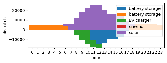
We can plot the dispatch of electricity from every generator throughout January 1st.

date="2015-07-01"
charge=n.storage_units_t.p['battery storage'][n.storage_units_t.p['battery storage']>0].loc[date]
discharge=n.storage_units_t.p['battery storage'][n.storage_units_t.p['battery storage']<0].loc[date]
EV_charge=n.links_t.p1['EV charger'].loc[date]
combined =  pd.concat([discharge, charge, EV_charge, n.generators_t.p.loc[date],], axis=1)
ax = combined.plot.bar(figsize=(6, 2), ylabel="dispatch", xlabel="hour", stacked=True, width=1)
ax.legend(loc='upper right')
ax.set_xticks(range(len(combined.index)))  
ax.set_xticklabels(combined.index.hour, rotation=0) 

[Text(0, 0, '0'),
 Text(1, 0, '1'),
 Text(2, 0, '2'),
 Text(3, 0, '3'),
 Text(4, 0, '4'),
 Text(5, 0, '5'),
 Text(6, 0, '6'),
 Text(7, 0, '7'),
 Text(8, 0, '8'),
 Text(9, 0, '9'),
 Text(10, 0, '10'),
 Text(11, 0, '11'),
 Text(12, 0, '12'),
 Text(13, 0, '13'),
 Text(14, 0, '14'),
 Text(15, 0, '15'),
 Text(16, 0, '16'),
 Text(17, 0, '17'),
 Text(18, 0, '18'),
 Text(19, 0, '19'),
 Text(20, 0, '20'),
 Text(21, 0, '21'),
 Text(22, 0, '22'),
 Text(23, 0, '23')]

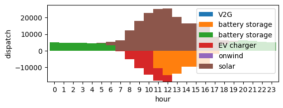
c) Assume that the EV batteries can also discharge into the grid. How do the required capacities change relative to section (a)? Plot the energy generation and demand throughout July 1st.

We can also allow vehicle-to-grid operation (i.e. electric vehicles can inject power back into the grid)

p_nom = number_cars * bev_charger_rate

n.add(
    "Link",
    "V2G",
    bus0="EV",
    bus1="electricity",
    p_nom=p_nom,
    p_max_pu=EV_availability_profile['PRT'].values,
    efficiency=0.9,
    overwrite=True,
)

Index(['V2G'], dtype='object', name='Link')

n.optimize(solver_name="highs")

WARNING:pypsa.consistency:The following generators have carriers which are not defined:
Index(['onwind', 'solar'], dtype='object', name='Generator')

WARNING:pypsa.consistency:The following stores have carriers which are not defined:
Index(['EV battery'], dtype='object', name='Store')

WARNING:pypsa.consistency:The following buses have carriers which are not defined:
Index(['electricity', 'EV'], dtype='object', name='Bus')

WARNING:pypsa.consistency:The following storage_units have carriers which are not defined:
Index(['battery storage'], dtype='object', name='StorageUnit')

WARNING:pypsa.consistency:The following links have carriers which are not defined:
Index(['EV charger', 'V2G'], dtype='object', name='Link')

INFO:linopy.model: Solve problem using Highs solver

INFO:linopy.io:Writing objective.

Writing constraints.:   0%|          | 0/19 [00:00<?, ?it/s]

Writing constraints.:  32%|███▏      | 6/19 [00:00<00:00, 47.10it/s]

Writing constraints.:  58%|█████▊    | 11/19 [00:00<00:00, 35.42it/s]

Writing constraints.:  79%|███████▉  | 15/19 [00:00<00:00, 33.61it/s]

Writing constraints.: 100%|██████████| 19/19 [00:00<00:00, 21.68it/s]

Writing constraints.: 100%|██████████| 19/19 [00:00<00:00, 25.97it/s]

Writing continuous variables.:   0%|          | 0/9 [00:00<?, ?it/s]

Writing continuous variables.:  78%|███████▊  | 7/9 [00:00<00:00, 64.99it/s]

Writing continuous variables.: 100%|██████████| 9/9 [00:00<00:00, 64.60it/s]

INFO:linopy.io: Writing time: 0.9s

Running HiGHS 1.10.0 (git hash: fd86653): Copyright (c) 2025 HiGHS under MIT licence terms
LP   linopy-problem-c996wgi4 has 175203 rows; 78843 cols; 319761 nonzeros
Coefficient ranges:
  Matrix [1e-03, 6e+00]
  Cost   [1e-02, 1e+05]
  Bound  [0e+00, 0e+00]
  RHS    [3e+02, 3e+05]
Presolving model
74478 rows, 74481 cols, 214674 nonzeros  0s

Dependent equations search running on 26280 equations with time limit of 1000.00s
Dependent equations search removed 0 rows and 0 nonzeros in 0.00s (limit = 1000.00s)
65718 rows, 65721 cols, 197154 nonzeros  0s
Presolve : Reductions: rows 65718(-109485); columns 65721(-13122); elements 197154(-122607)
Solving the presolved LP
Using EKK dual simplex solver - serial
  Iteration        Objective     Infeasibilities num(sum)
          0     3.3633085259e+02 Pr: 17520(8.09173e+08) 0s

      77156     6.5753106576e+09 Pr: 0(0); Du: 1088(0.459153) 6s

      79836     6.5753004797e+09 Pr: 0(0); Du: 0(4.54747e-13) 7s
      79836     6.5753004797e+09 Pr: 0(0); Du: 0(4.54747e-13) 7s
Solving the original LP from the solution after postsolve
Model name          : linopy-problem-c996wgi4
Model status        : Optimal
Simplex   iterations: 79836
Objective value     :  6.5753004797e+09
Relative P-D gap    :  1.3053500557e-15
HiGHS run time      :          7.41

INFO:linopy.constants: Optimization successful: 
Status: ok
Termination condition: optimal
Solution: 78843 primals, 175203 duals
Objective: 6.58e+09
Solver model: available
Solver message: Optimal

INFO:pypsa.optimization.optimize:The shadow-prices of the constraints Generator-ext-p-lower, Generator-ext-p-upper, Link-fix-p-lower, Link-fix-p-upper, Store-fix-e-lower, Store-fix-e-upper, StorageUnit-ext-p_dispatch-lower, StorageUnit-ext-p_dispatch-upper, StorageUnit-ext-p_store-lower, StorageUnit-ext-p_store-upper, StorageUnit-ext-state_of_charge-lower, StorageUnit-ext-state_of_charge-upper, StorageUnit-energy_balance, Store-energy_balance were not assigned to the network.

Writing the solution to /tmp/linopy-solve-npq2d9jx.sol

('ok', 'optimal')

n.objective / 1e9

6.5753004796690036

n.objective/n.loads_t.p_set.sum().sum()

np.float64(96.16212998126574)

n.generators.p_nom_opt.div(1e3)  # MW -> GW

Generator
onwind    24.867237
solar     49.156260
Name: p_nom_opt, dtype: float64

n.storage_units.max_hours*n.storage_units.p_nom_opt.div(1e3) #MWh - GWh

StorageUnit
battery storage    88.438146
dtype: float64

Similarly to section b, here the cost of every MWh or electricity generated is even lower and this is mainly because with the EV batteries allowing discharging back into the grid (vehicle-to-grid), the need for static batteries is further reduced.

The cost of every MWh or electricity generated is lower and this is mainly becuase with the EV battery, the need for static batteries is significantly reduced

n.generators_t.p.sum().div(1e6)  # MWh -> TWh

Generator
onwind     8.061303
solar     64.202418
dtype: float64

We can plot the dispatch of electricity from every generator throughout January 1st.

date="2015-07-01"
charge = n.storage_units_t.p['battery storage'][n.storage_units_t.p['battery storage']>0].loc[date]
discharge = n.storage_units_t.p['battery storage'][n.storage_units_t.p['battery storage']<0].loc[date]
EV_charge = n.links_t.p1['EV charger'].loc[date]
EV_discharge = -n.links_t.p1['V2G'].loc[date]
combined =  pd.concat([EV_discharge, discharge, charge, EV_charge, n.generators_t.p.loc[date],], axis=1)
ax = combined.plot.bar(figsize=(6, 2), ylabel="dispatch", xlabel="hour", stacked=True, width=1)
ax.legend(loc='upper right')
ax.set_xticks(range(len(combined.index)))  
ax.set_xticklabels(combined.index.hour, rotation=0)  

[Text(0, 0, '0'),
 Text(1, 0, '1'),
 Text(2, 0, '2'),
 Text(3, 0, '3'),
 Text(4, 0, '4'),
 Text(5, 0, '5'),
 Text(6, 0, '6'),
 Text(7, 0, '7'),
 Text(8, 0, '8'),
 Text(9, 0, '9'),
 Text(10, 0, '10'),
 Text(11, 0, '11'),
 Text(12, 0, '12'),
 Text(13, 0, '13'),
 Text(14, 0, '14'),
 Text(15, 0, '15'),
 Text(16, 0, '16'),
 Text(17, 0, '17'),
 Text(18, 0, '18'),
 Text(19, 0, '19'),
 Text(20, 0, '20'),
 Text(21, 0, '21'),
 Text(22, 0, '22'),
 Text(23, 0, '23')]