Problem 3.3

Integrated Energy Grids

Problem 3.3

Using the Python package networkX, codify the network described in Problem 3.2

Note

If you have not yet set up Python on your computer, you can execute this tutorial in your browser via Google Colab. Click on the rocket in the top right corner and launch “Colab”. If that doesn’t work download the .ipynb file and import it in Google Colab.

Then install the following packages by executing the following command in a Jupyter cell at the top of the notebook.

!pip install numpy networkx pandas matplotlib

We start by creating the network and adding the nodes and links.

N = nx.Graph()
N.add_nodes_from([0, 1, 2, 3, 4])
N.add_edges_from([(0, 1), (1, 2), (1, 3), (1, 4), (2,4)])

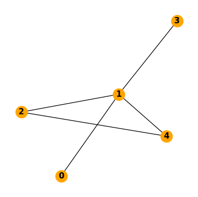
a) Make a plot of the network

fig, ax = plt.subplots(figsize=(5, 5))
nx.draw(N, with_labels=True, ax=ax, node_color="orange", font_weight="bold")

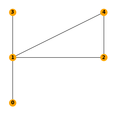
We can add the position of every node to make the figure more similar to the original plot.

pos=nx.get_node_attributes(N,'pos')
pos[0] = np.array([0, 0])
pos[1] = np.array([0, 1])
pos[2] = np.array([1, 1])
pos[3] = np.array([0, 2])
pos[4] = np.array([1, 2])

fig, ax = plt.subplots(figsize=(5, 5))
nx.draw(N, with_labels=True, ax=ax, pos=pos, node_color="orange", font_weight="bold")

b) Calculate the degree in every node and the average degree

degrees=[deg for node, deg in N.degree()]
np.mean(degrees)

np.float64(2.0)

c) Calculate the Degree, Adjacency, Incidence and Laplacian matrix. Make a heat-map of each of those matrices to evaluate them visually.

Degree matrix

D = np.diag(degrees)

plt.imshow(D, cmap="Blues")

<matplotlib.image.AxesImage at 0x7fb8da09ea10>

Adjacency matrix (Careful, networkx will yield a weighted adjacency matrix by default!)

A = nx.adjacency_matrix(N, weight=None).todense()

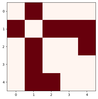
We can plot the matrix to get a visual overview of how interconnected is the network

plt.imshow(A, cmap="Reds")

<matplotlib.image.AxesImage at 0x7fb8da02b750>

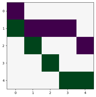
Incidence matrix (Careful, networkx will yield a incidence matrix without orientation by default!)

K=nx.incidence_matrix(N, oriented=True).todense()
K

array([[-1.,  0.,  0.,  0.,  0.],
       [ 1., -1., -1., -1.,  0.],
       [ 0.,  1.,  0.,  0., -1.],
       [ 0.,  0.,  1.,  0.,  0.],
       [ 0.,  0.,  0.,  1.,  1.]])

plt.imshow(K, cmap="PRGn")

<matplotlib.image.AxesImage at 0x7fb8c9ad8ed0>

Laplacian matrix (Careful, networkx will yield a weighted Laplacian matrix by default!)

L = nx.laplacian_matrix(N, weight=None).todense()
L

array([[ 1, -1,  0,  0,  0],
       [-1,  4, -1, -1, -1],
       [ 0, -1,  2,  0, -1],
       [ 0, -1,  0,  1,  0],
       [ 0, -1, -1,  0,  2]])

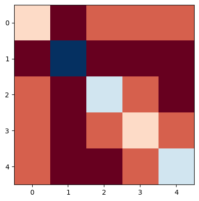
plt.imshow(L, cmap="RdBu")

<matplotlib.image.AxesImage at 0x7fb8c9b0ea10>