Problem 2.2

Problem 2.2#

Integrated Energy Grids

Problem 2.2

Consider the following economic dispatch problem:

we have three generators: solar, wind and gas
solar and wind have no marginal costs, and gas has fuel costs of 60 EUR/MWh.
we need to cover demand of 13.2 MWh
the installed capacities are 15 MW, 20 MW and 20 MW for wind, solar, and gas, respectively
assume the capacity factor for solar is 0.17 and for wind 0.33.

a) Use linopy to define and solve the LP and find the optimal solution as well as reading out the Lagrange multipliers as defined in the lecture.

b) Open problem2_2b.csv, and use the values as inputs for capacity factors as well as demand in the dispatch problem. Solve the LP with linopy.

c) Open problem2_2c.csv, and use the values as inputs for capacity factors as well as demand in the dispatch problem. Solve the LP with linopy.

d) Compare the share of renewable generation, the dual variables, and the objective from a)-c) [average, median, min, max] and interpret the differences. Compute the curtailment from renewables.

e) Plot the supply and demand duration curves for the different resources in c). Also consider demand - renewable generation (“net load”). Could transmission or storage be useful for this system? Why or why not?

We will use numpy to operate with arrays and matplotlib.pyplot to plot the results. We also use linopy to solve linear problems and work with pandas to work with dataframes.

import pandas as pd
import numpy as np
import linopy 
import matplotlib.pyplot as plt

a)

Define the capacities of the generators.

# Installed capacities
wind = 15
solar = 20
gas = 20

Set the marginal costs of gas.

# Marginal costs (for solar and wind 0)
cost_gas = 60

Fix demand and capacity factors.

# Fixed demand
demand_2a = 13.2

# Capacity factors
solar_cf = 0.17
wind_cf = 0.33

Set up the minimization problem in linopy.

Print the duals

b)

Read the data for problem 2b.

problem2b = pd.read_csv("./data/problem2_2b.csv", index_col=0, parse_dates=True)

Define the model. Note that there is a time dimension to the data we loaded, so add a time coordinate to the variables

Compute the duals

c)

Load the data for problem 2c.

problem2c = pd.read_csv("./data/problem2_2c.csv", index_col=0, parse_dates=True)

As above set up the linopy model.

Compute the duals

d)

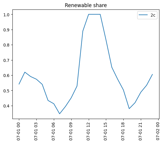
Compute the renewable share in the production as the wind and solar generation in each hour divided by the demand. Plot the time series from 2c in matplotlib.pyplot.

# Renewable share
fig, ax = plt.subplots()

renewable_share_2a = (m22.solution["wind"] + m22.solution["solar"] )/ demand_2a
renewable_share_2b = pd.Series(data=(m22b.solution["wind"] + m22b.solution["solar"]) / problem2b["demand [MWh]"], index=problem2b.index)
renewable_share_2c = pd.Series(data=(m22c.solution["wind"] + m22c.solution["solar"]) / problem2c["demand [MWh]"], index=problem2c.index)


ax.plot(renewable_share_2c, label="2c");
ax.set_title("Renewable share");
ax.set_xticklabels(ax.get_xticklabels(), rotation=90);
ax.legend();

/tmp/ipykernel_2242/135273699.py:11: UserWarning: set_ticklabels() should only be used with a fixed number of ticks, i.e. after set_ticks() or using a FixedLocator.
  ax.set_xticklabels(ax.get_xticklabels(), rotation=90);

../_images/a8b7995db50792f0d58785c7d79aaf34870e29f9b39b1fb962693f0ecaace250.png

print("Renewable share 2a: ", renewable_share_2a.values)
print("Renewable share 2b: ", renewable_share_2b.mean())
print("Renewable share 2c: ", renewable_share_2c.mean())

Renewable share 2a:  0.6325757575757576
Renewable share 2b:  0.6047916805148708
Renewable share 2c:  0.5962939748513115

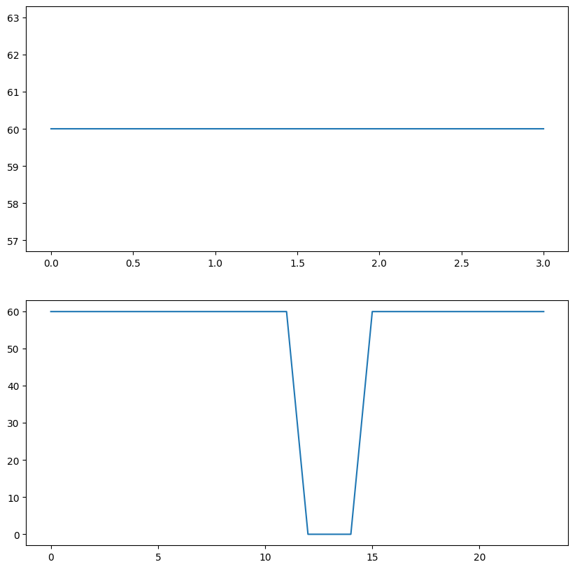
Plot the dual variables / electricity prices from b and c, and print them for a

fig, axs = plt.subplots(2,1, figsize=(10,10))

axs[0].plot(m22b.dual.energy_balance, label="Electricity price (b)")
axs[1].plot(m22c.dual.energy_balance, label="Electricity price (c)")


print("Electricity price (a):", m22.dual.energy_balance.values.mean())
print("Electricity price (b):", m22b.dual.energy_balance.to_pandas().describe())
print("Electricity price (c):", m22c.dual.energy_balance.to_pandas().describe())

Electricity price (a): 60.0
Electricity price (b): count     4.0
mean     60.0
std       0.0
min      60.0
25%      60.0
50%      60.0
75%      60.0
max      60.0
Name: energy_balance, dtype: float64
Electricity price (c): count    24.000000
mean     52.500000
std      20.269918
min       0.000000
25%      60.000000
50%      60.000000
75%      60.000000
max      60.000000
Name: energy_balance, dtype: float64

../_images/d7f00c41d00ff815051a220f9d446df68fb10abd1fceddb5db2d8bd5f2a96117.png

Compare the objective from a to c as well as the average cost per hour. Note that with higher detail and higher spatial resolution of the renewables the costs increase on average (even more so for the objective which has more time steps). This is because fluctuations in generations are less smoothed.

print("Objective 2a: ", m22.objective.value, " and average cost per hour: ", m22.objective.value)
print("Objective 2b: ", m22b.objective.value, " and average cost per hour: ", m22b.objective.value/len(problem2b))
print("Objective 2c: ", m22c.objective.value, " and average cost per hour: ", m22c.objective.value/len(problem2c))

Objective 2a:  290.99999999999994  and average cost per hour:  290.99999999999994
Objective 2b:  1220.4  and average cost per hour:  305.1
Objective 2c:  7695.0  and average cost per hour:  320.625

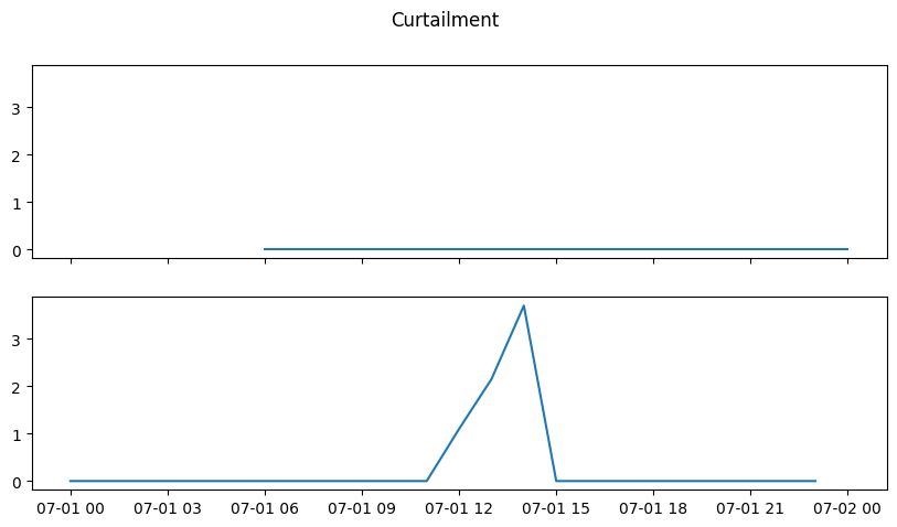
Print curtailment as the difference between renewable potential (capacity factor * capacity) for each hour and the renewable generation in the solutions.

# Curtailment
fig, ax = plt.subplots(2,1, figsize=(10,5), sharex=True, sharey=True)

ren_pot_2b = solar * problem2b["solar cf"] + wind * problem2b["wind cf"]
ren_pot_2c = solar * problem2c["solar cf"] + wind * problem2c["wind cf"]

curtailment_2b = ren_pot_2b - (m22b.solution["wind"] + m22b.solution["solar"])
curtailment_2c = ren_pot_2c - (m22c.solution["wind"] + m22c.solution["solar"])

ax[0].plot(curtailment_2b, label="2b")
ax[1].plot(curtailment_2c, label="2c")

fig.suptitle("Curtailment");

../_images/923208bcc5ee8432df0d996538ca862d860e8a5edf4f5801c872a9daaf93aeca.png

e)

Plot the supply duration curves by sorting the generation for each technology (and resetting the index). Do the same for the demand.

Compute net load as the difference of renewable generation and demand.

# Plot supply curves from c)

fig, axs = plt.subplots(1,2, figsize=(15,5))

ax = axs[0]
ax.set_title(f"Supply and demand duration curves")

ax.plot(m22c.solution.wind.to_pandas().sort_values(ascending=False).reset_index(drop=True), label="Wind")
ax.plot(m22c.solution.solar.to_pandas().sort_values(ascending=False).reset_index(drop=True), label="Solar")
ax.plot(m22c.solution.gas.to_pandas().sort_values(ascending=False).reset_index(drop=True), label="Gas")
ax.plot(problem2c["demand [MWh]"].sort_values(ascending=False).reset_index(drop=True), label="Demand")

ax.legend()

ax = axs[1]
ax.set_title(f"Net load")
ax.plot((problem2c["solar cf"] * solar + problem2c["wind cf"] * wind - problem2c["demand [MWh]"]).sort_values(ascending=False).reset_index(drop=True), label="Net load")
ax.hlines(0, 0, 24, color="grey")

ax.legend()

<matplotlib.legend.Legend at 0x7f35d31be7d0>

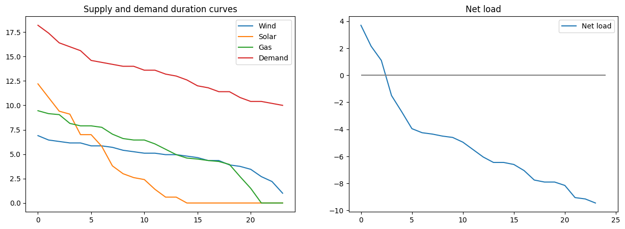
../_images/010cf2172938376fe153f57e8c0968be972ea60a8fdb9bc5497546a65b56a670.png

We have some curtailment as seen in d), so for the few hours of surplus it would be useful to smooth production in one way or another, either through transmission, or storage, or demand response.