Problem 4.3

Integrated Energy Grids

Problem 4.3

Note

If you have not yet set up Python on your computer, you can execute this tutorial in your browser via Google Colab. Click on the rocket in the top right corner and launch “Colab”. If that doesn’t work download the .ipynb file and import it in Google Colab.

Then install the following packages by executing the following command in a Jupyter cell at the top of the notebook.

!pip install numpy networkx pandas matplotlib

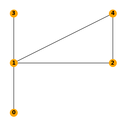
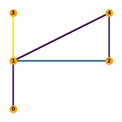
We start by creating the network and adding the nodes and links.

N = nx.Graph()
N.add_nodes_from([0, 1, 2, 3, 4])
N.add_edges_from([(0, 1), (1, 2), (1, 3), (1, 4), (2,4)])

pos=nx.get_node_attributes(N,'pos')
pos[0] = np.array([0, 0])
pos[1] = np.array([0, 1])
pos[2] = np.array([1, 1])
pos[3] = np.array([0, 2])
pos[4] = np.array([1, 2])

fig, ax = plt.subplots(figsize=(5, 5))
nx.draw(N, with_labels=True, ax=ax, pos=pos, node_color="orange", font_weight="bold")

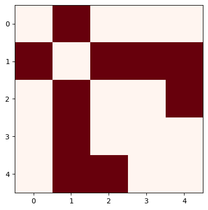
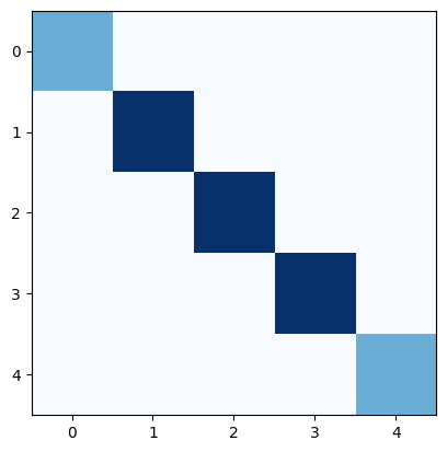
c) Calculate the Degree, Adjacency, Incidence, and Laplacian matrix

Adjacency matrix (Careful, networkx will yield a weighted adjacency matrix by default!)

A = nx.adjacency_matrix(N, weight=None).todense()

We can plot the matrix to get a visual overview of how interconnected is the network

plt.imshow(A, cmap="Reds")

<matplotlib.image.AxesImage at 0x7f41cd2b38d0>

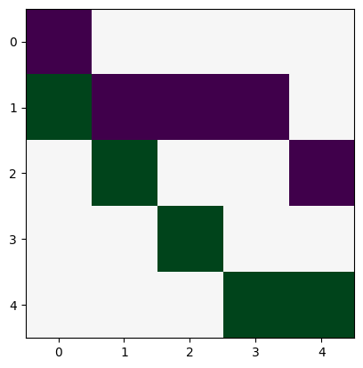
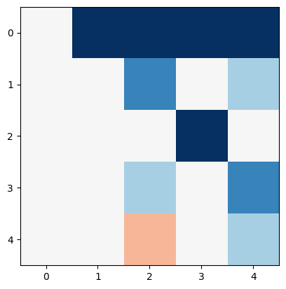
incidence matrix (Careful, networkx will yield a incidence matrix without orientation by default!)

K=nx.incidence_matrix(N, oriented=True).todense()
K

array([[-1.,  0.,  0.,  0.,  0.],
       [ 1., -1., -1., -1.,  0.],
       [ 0.,  1.,  0.,  0., -1.],
       [ 0.,  0.,  1.,  0.,  0.],
       [ 0.,  0.,  0.,  1.,  1.]])

plt.imshow(K, cmap="PRGn")

<matplotlib.image.AxesImage at 0x7f41bf7a1b50>

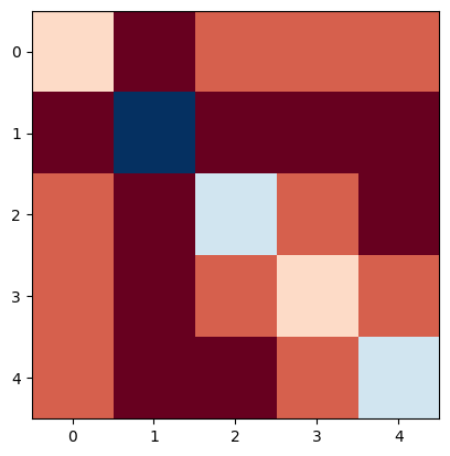
Laplacian matrix (Careful, networkx will yield a weighted adjacency matrix by default!)

L = nx.laplacian_matrix(N, weight=None).todense()
L

array([[ 1, -1,  0,  0,  0],
       [-1,  4, -1, -1, -1],
       [ 0, -1,  2,  0, -1],
       [ 0, -1,  0,  1,  0],
       [ 0, -1, -1,  0,  2]])

plt.imshow(L, cmap="RdBu")

<matplotlib.image.AxesImage at 0x7f41bf7d4d50>

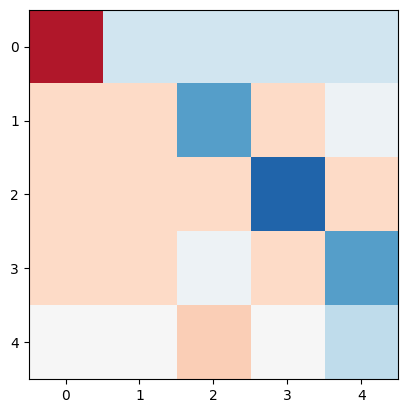
a) Assuming that the reactance in the links is \(x_l\)=1, calculate the Power Transfer Distribution Factor (PTDF) matrix

The PTDF matrix measures the sensitivity of power flows in each transmission line relative to incremental changes in nodal power injections or withdrawals throughout the electricity network.

\[p_\ell = \frac{1}{x_\ell}\sum_{i,j} K_{i\ell} (L^{-1})_{ij} p_j\]

\[p_\ell = \sum_j \text{PTDF}_{\ell j} p_j\]

The weighted Laplacian of the network is not invertible, but we can use the Moore Penrose pseudo-inverse

L_inv = np.linalg.pinv(L)

or apply a trick by disregarding the first column and row of the weighted Laplacian for inversion:

n_nodes = L.shape[0]

L_inv = np.linalg.inv(L[1:, 1:])
L_inv = np.hstack((np.zeros((n_nodes - 1, 1)), L_inv))
L_inv = np.vstack((np.zeros(n_nodes), L_inv))

Now, we can calculate the PTDF matrix

PTDF = K.T.dot(L_inv)

plt.imshow(PTDF, cmap="RdBu", vmin=-1, vmax=1)

<matplotlib.image.AxesImage at 0x7f41bf869b50>

b) Assuming the power injection pattern described in Problem 4.1 determine the power flows in the lines of the network and plot them.

p_i =[-2, 5, 6, -8, -1]
p_l = PTDF.dot(p_i)
p_l

array([ 2.        ,  3.66666667, -8.        ,  1.33333333, -2.33333333])

abs_p_l = np.abs(p_l)
fig, ax = plt.subplots(figsize=(5, 5))
nx.draw(N, 
        with_labels=True, 
        ax=ax, 
        pos=pos, 
        node_color="orange", 
        font_weight="bold",  
        edge_color=abs_p_l, 
        width=4)

c) Assume now that the links unitary susceptance is \(x_{l}\)=[1, 0.5, 0.5, 0.5, 1], calculate the weighted Laplacian (or susceptance matrix), the PTDF matrix, the power flows and plot them.

If we want to calculate the weighted Laplacian \(L = KBK^\top\), we also need the diagonal matrix \(B\) for the susceptances (i.e inverse of reactances; \(1/x_\ell\)):

x_pu = [1, 0.5, 0.5, 0.5, 1]
b = [1 / x for x in x_pu]

B = np.diag(b)

plt.imshow(B, cmap="Blues") 

<matplotlib.image.AxesImage at 0x7f41bf97add0>

Now, we can calculate the weighted Laplacian as \(K_{il}\frac{1}{x_l}K_{lj}\)

L = K.dot(B.dot(K.T))
L

array([[ 1., -1.,  0.,  0.,  0.],
       [-1.,  7., -2., -2., -2.],
       [ 0., -2.,  3.,  0., -1.],
       [ 0., -2.,  0.,  2.,  0.],
       [ 0., -2., -1.,  0.,  3.]])

We can invert the Laplacian and multiply by the transpose of the incidence matrix to create the PTDF matrix.

L_inv = np.linalg.pinv(L)

PTDF = (B.dot(K.T)).dot(L_inv)

plt.imshow(PTDF, cmap="RdBu", vmin=-1, vmax=1)

<matplotlib.image.AxesImage at 0x7f41bf6a6290>

And calculate the flows thrgoughout the lines

p_l=PTDF.dot(p_i)
p_l

array([ 2.  ,  4.25, -8.  ,  0.75, -1.75])